2 Newton’s method for minimization
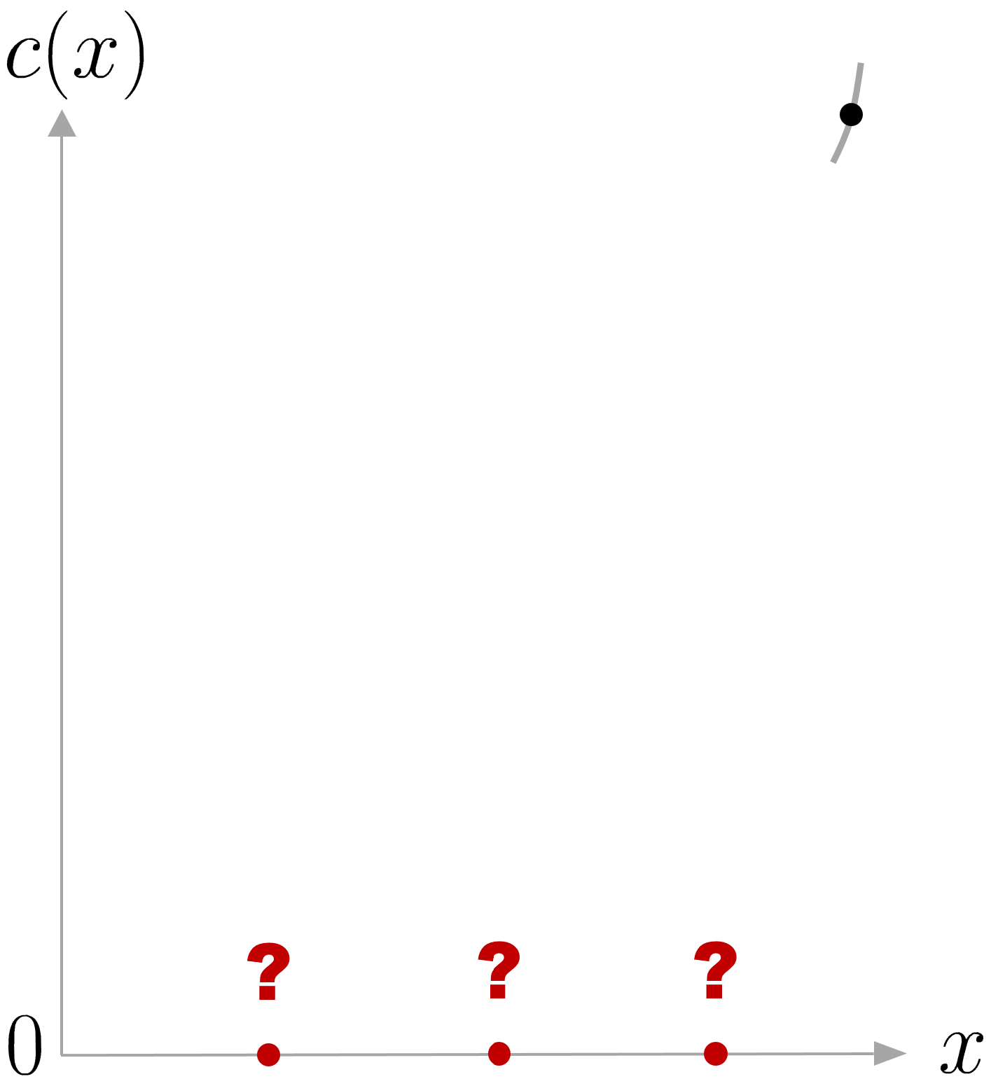
We would like the find the value of a decision variable x that would give us a cost c(x) that is a small as possible, see Figure 1 . Imagine that we start from an initial guess x_{1} and that can observe the behavior of this cost function within a very small region around our initial guess. Now let’s assume that we can make several consecutive guesses that will each time provide us with similar local information about the behavior of the cost around the points that we guessed. From this information, what point would you select as second guess (see question marks in the figure), based on the information that you obtained from the first guess? There were two relevant information in the small portion of curve that we can observe in the figure to make a smart choice. First, the trend of the curve indicates that the cost seems to decrease if we move on the left side, and increase if we move on the right side. Namely, the slope c^{\prime}(x_{1}) of the function c(x) at point x_{1} is positive. Second, we can observe that the portion of the curve has some curvature that can be also be informative about the way the trend of the curve c(x) will change by moving to the left or to the right. Namely, how much the slope c^{\prime}(x_{1}) will change, corresponding to an acceleration c^{\prime\prime}(x_{1}) around our first guess x_{1} . This is informative to estimate how much we should move to the left of the first guess to wisely select a second guess.
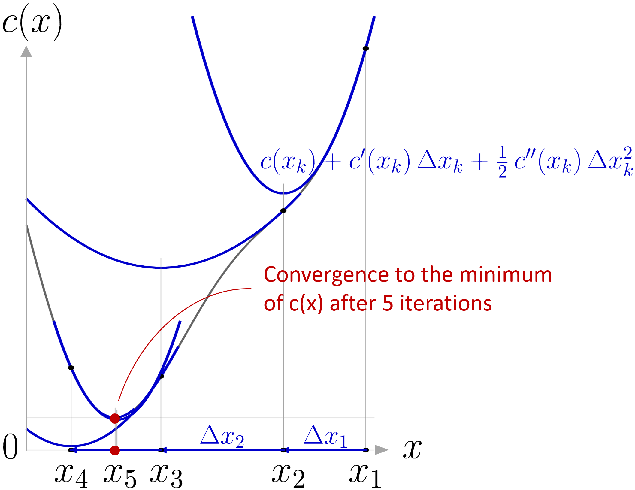
Now that we have this intuition, we can move to a more formal problem formulation. Newton’s method attempts to solve \min_{x}c(x) or \max_{x}c(x) from an initial guess x_{1} by using a sequence of second-order Taylor approximations of c(x) around the iterates, see Fig. 2 .
The second-order Taylor expansion around the point x_{k} can be expressed as
| c(x_{k}\!+\!\Delta x_{k})\approx c(x_{k})+c^{\prime}(x_{k})\;\Delta x_{k}+\frac{1}{2}c^{\prime\prime}(x_{k})\;\Delta x_{k}^{2}, |
where c^{\prime}(x_{k}) and c^{\prime\prime}(x_{k}) are the first and second derivatives at point x_{k} .
We are interested in solving minimization problems with this approximation. If the second derivative c^{\prime\prime}(x_{k}) is positive, the quadratic approximation is a convex function of \Delta x_{k} , and its minimum can be found by setting the derivative to zero.
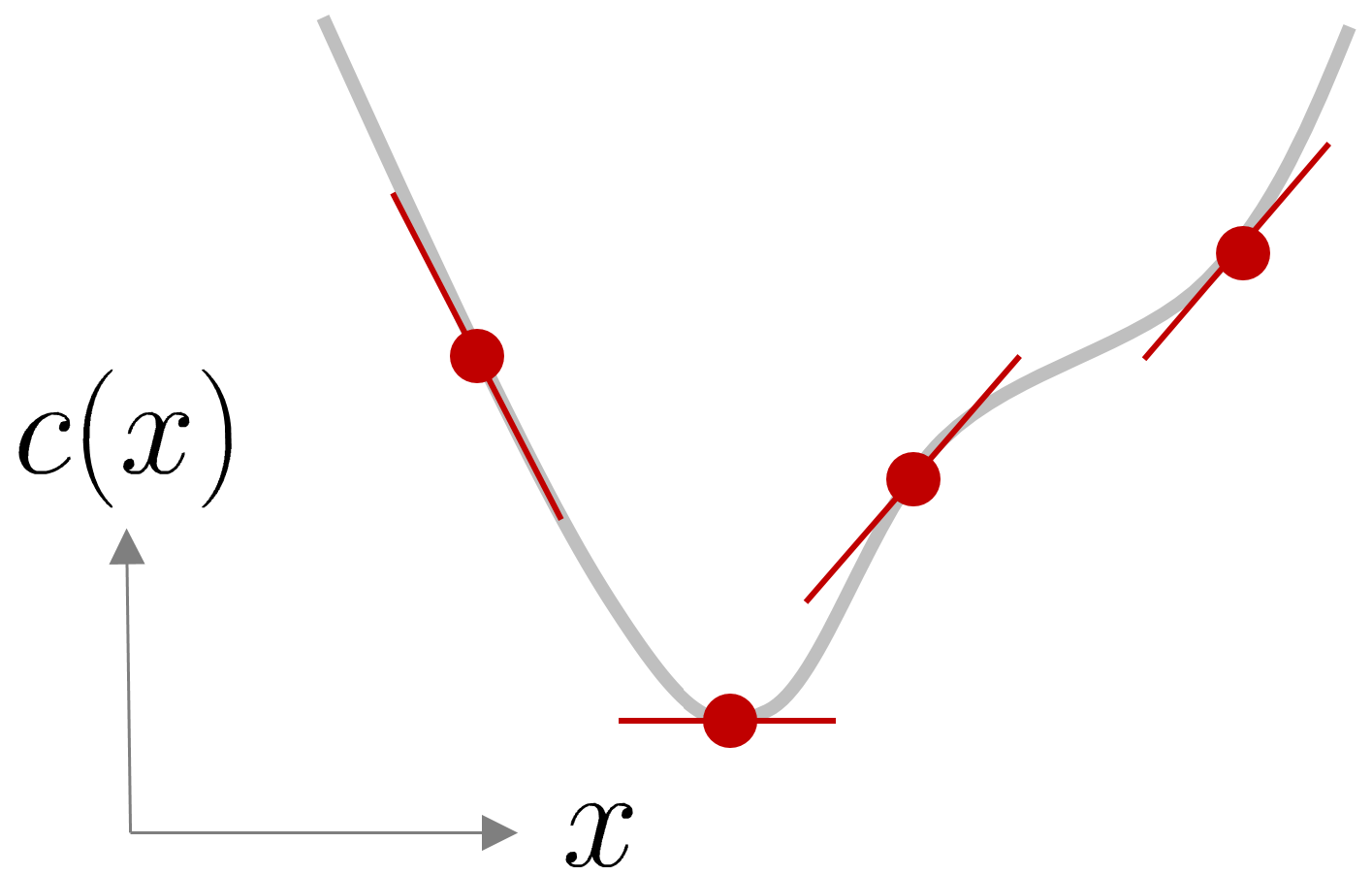
To find the local optima of a function, we can localize the points whose derivatives are zero, see Figure 3 for an illustration.
Thus, by differentiating ( 1 ) w.r.t. \Delta x_{k} and equating to zero, we obtain
| c^{\prime}(x_{k})+c^{\prime\prime}(x_{k})\,\Delta x_{k}=0, |
meaning that the minimum is given by
| \Delta\hat{x}_{k}=-\frac{c^{\prime}(x_{k})}{c^{\prime\prime}(x_{k})} |
which corresponds to the offset to apply to x_{k} to minimize the second-order polynomial approximation of the cost at this point.
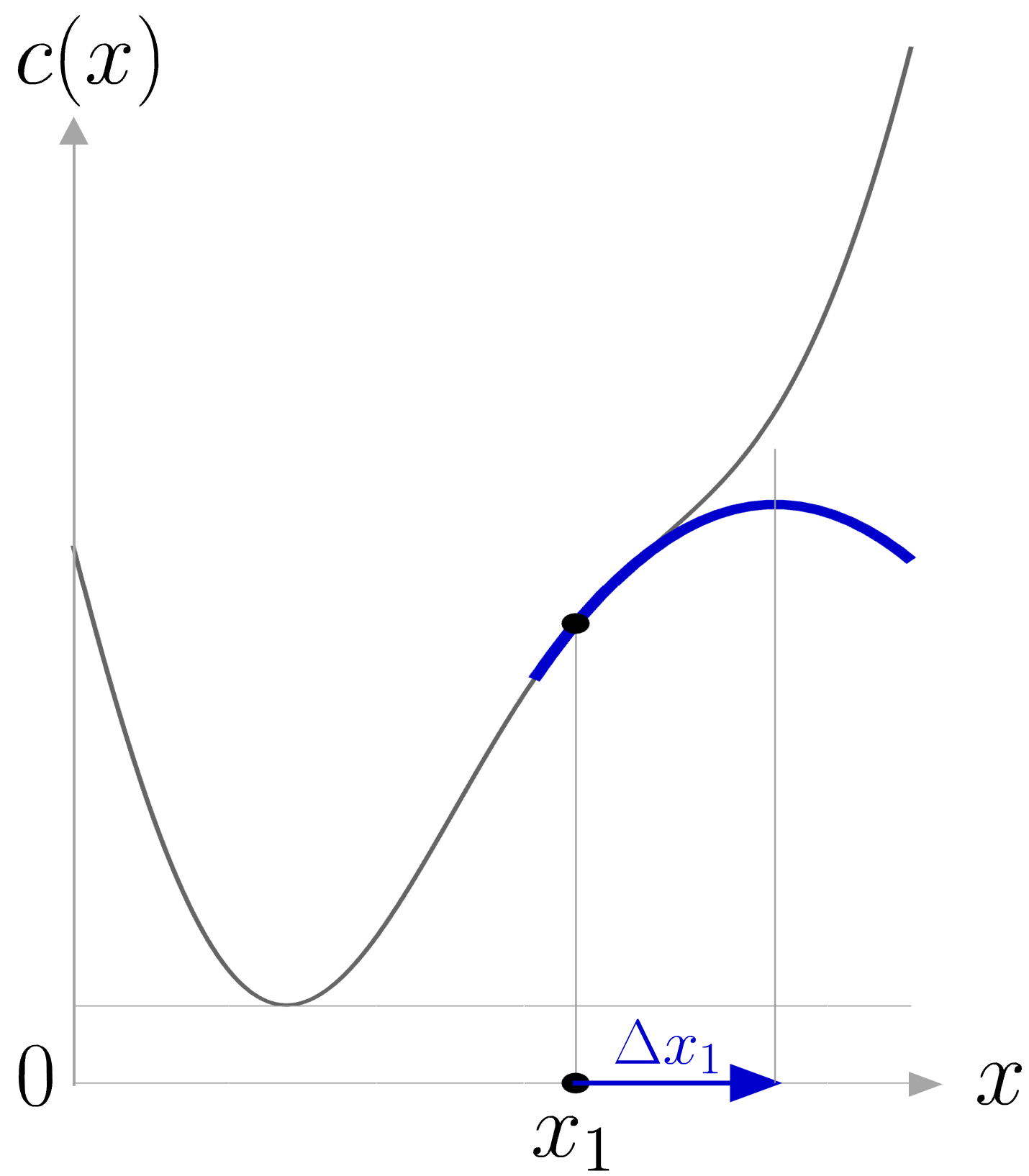
It is important that c^{\prime\prime}(x_{k}) is positive if we want to find local minima, see Figure 4 for an illustration.
By starting from an initial estimate x_{1} and by recursively refining the current estimate by computing the offset that would minimize the polynomial approximation of the cost at the current estimate, we obtain at each iteration k the recursion
| x_{k+1}=x_{k}-\frac{c^{\prime}(x_{k})}{c^{\prime\prime}(x_{k})}. |
The geometric interpretation of Newton’s method is that at each iteration, it amounts to the fitting of a paraboloid to the surface of c(x) at x_{k} , having the same slopes and curvature as the surface at that point, and then proceeding to the maximum or minimum of that paraboloid. Note that if c(x) is a quadratic function, then the exact extremum is found in one step, which corresponds to the resolution of a least-squares problem.
Multidimensional case
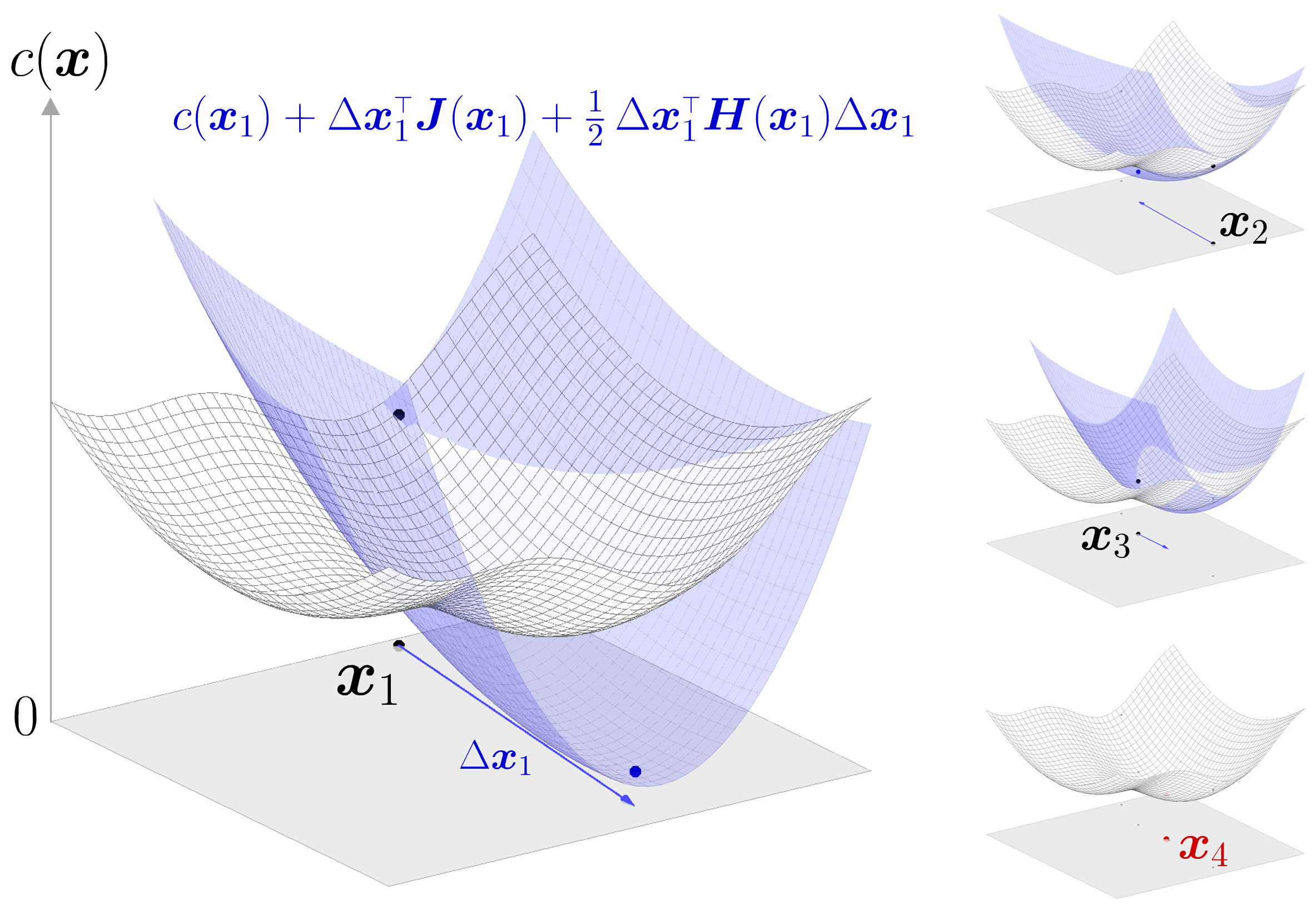
For functions that depend on multiple variables stored as multidimensional vectors \bm{x} , the cost function c(\bm{x}) can similarly be approximated by a second-order Taylor expansion around the point \bm{x}_{k} with
| c(\bm{x}_{k}\!+\!\Delta\bm{x}_{k})\approx c(\bm{x}_{k})+\Delta\bm{x}_{k}^{\scriptscriptstyle\top}\,\frac{\partial c}{\partial\bm{x}}\Big|_{\bm{x}_{k}}+\frac{1}{2}\Delta\bm{x}_{k}^{\scriptscriptstyle\top}\,\frac{\partial^{2}c}{\partial\bm{x}^{2}}\Big|_{\bm{x}_{k}}\Delta\bm{x}_{k}, |
which can also be rewritten in augmented vector form as
| c(\bm{x}_{k}\!+\!\Delta\bm{x}_{k})\approx c(\bm{x}_{k})+\frac{1}{2}\begin{bmatrix}1\\ \Delta\bm{x}_{k}\end{bmatrix}^{\!{\scriptscriptstyle\top}}\begin{bmatrix}0&\bm{g}_{\bm{x}}^{\scriptscriptstyle\top}\\ \bm{g}_{\bm{x}}&\bm{H}_{\bm{x}\bm{x}}\end{bmatrix}\begin{bmatrix}1\\ \Delta\bm{x}_{k}\end{bmatrix}, |
with gradient vector
| \bm{g}(\bm{x}_{k})=\frac{\partial c}{\partial\bm{x}}\Big|_{\bm{x}_{k}}, |
and Hessian matrix
| \bm{H}(\bm{x}_{k})=\frac{\partial^{2}c}{\partial\bm{x}^{2}}\Big|_{\bm{x}_{k}}. |
We are interested in solving minimization problems with this approximation. If the Hessian matrix \bm{H}(\bm{x}_{k}) is positive definite, the quadratic approximation is a convex function of \Delta\bm{x}_{k} , and its minimum can be found by setting the derivatives to zero, see Figure 5 .
By differentiating ( 3 ) w.r.t. \Delta\bm{x}_{k} and equation to zero, we obtain that
| \Delta\bm{\hat{x}}_{k}=-{\bm{H}(\bm{x}_{k})}^{-1}\,\bm{g}(\bm{x}_{k}), |
is the offset to apply to \bm{x}_{k} to minimize the second-order polynomial approximation of the cost at this point.
By starting from an initial estimate \bm{x}_{1} and by recursively refining the current estimate by computing the offset that would minimize the polynomial approximation of the cost at the current estimate, we obtain at each iteration k the recursion
| \bm{x}_{k+1}=\bm{x}_{k}-{\bm{H}(\bm{x}_{k})}^{-1}\,\bm{g}(\bm{x}_{k}). |
2.1 Gauss–Newton algorithm
The Gauss–Newton algorithm is a special case of Newton’s method in which the cost is quadratic (sum of squared function values), with c(\bm{x})=\sum_{i=1}^{R}r_{i}^{2}(\bm{x})=\bm{r}^{\scriptscriptstyle\top}\bm{r} , where \bm{r} are residual vectors. We neglect in this case the second-order derivative terms of the Hessian. The gradient and Hessian can in this case be computed with
| \bm{g}=2\bm{J}_{\bm{r}}^{\scriptscriptstyle\top}\bm{r},\quad\bm{H}\approx 2\bm{J}_{\bm{r}}^{\scriptscriptstyle\top}\bm{J}_{\bm{r}}, |
where \bm{J}_{\bm{r}}\in\mathbb{R}^{R\times D} is the Jacobian matrix of \bm{r}\in\mathbb{R}^{R} . This definition of the Hessian matrix makes it positive definite, which is useful to solve minimization problems as for well conditioned Jacobian matrices, we do not need to verify the positive definiteness of the Hessian matrix at each iteration.
The update rule in ( 6 ) then becomes
| \displaystyle\bm{x}_{k+1} | \displaystyle=\bm{x}_{k}-{\big(\bm{J}_{\bm{r}}^{\scriptscriptstyle\top}(\bm{x}_{k})\bm{J}_{\bm{r}}(\bm{x}_{k})\big)}^{-1}\,\bm{J}_{\bm{r}}^{\scriptscriptstyle\top}(\bm{x}_{k})\,\bm{r}(\bm{x}_{k}) | ||
| \displaystyle=\bm{x}_{k}-\bm{J}_{\bm{r}}^{\dagger}(\bm{x}_{k})\,\bm{r}(\bm{x}_{k}), |
where \bm{J}_{\bm{r}}^{\dagger} denotes the pseudoinverse of \bm{J}_{\bm{r}} .
The Gauss–Newton algorithm is the workhorse of many robotics problems, including inverse kinematics and optimal control, as we will see in the next sections.
2.2 Least squares
When the cost c(\bm{x}) is a quadratic function w.r.t. \bm{x} , the optimization problem can be solved directly, without requiring iterative steps. Indeed, for any matrix \bm{A} and vector \bm{b} , we can see that if
| c(\bm{x})=(\bm{A}\bm{x}-\bm{b})^{\scriptscriptstyle\top}(\bm{A}\bm{x}-\bm{b}), |
derivating c(\bm{x}) w.r.t. \bm{x} and equating to zero yields
| \bm{A}\bm{x}-\bm{b}=\bm{0}\iff\bm{x}=\bm{A}^{\dagger}\bm{b}, |
which corresponds to the standard analytic least squares estimate. We will see later in the inverse kinematics section that for the complete solution can also include a nullspace structure.
2.3 Least squares with constraints
A constrained minimization problem of the form
| \min_{\bm{x}}\;(\bm{A}\bm{x}-\bm{b})^{\scriptscriptstyle\top}(\bm{A}\bm{x}-\bm{b}),\quad\text{s.t.}\quad\bm{C}\bm{x}=\bm{h}, |
can also be solved analytically by considering a Lagrange multiplier variable \bm{\lambda} allowing us to rewrite the objective as
| \min_{\bm{x},\bm{\lambda}}\;(\bm{A}\bm{x}-\bm{b})^{\scriptscriptstyle\top}(\bm{A}\bm{x}-\bm{b})+\bm{\lambda}^{\scriptscriptstyle\top}(\bm{C}\bm{x}-\bm{h}). |
Differentiating with respect to \bm{x} and \bm{\lambda} and equating to zero yields
| \bm{A}^{\scriptscriptstyle\top}(\bm{A}\bm{x}-\bm{b})+\bm{C}^{\scriptscriptstyle\top}\bm{\lambda}=\bm{0},\quad\bm{C}\bm{x}-\bm{h}=\bm{0}, |
which can rewritten in matrix form as
| \begin{bmatrix}\bm{A}^{\scriptscriptstyle\top}\!\bm{A}&\bm{C}^{\scriptscriptstyle\top}\\ \bm{C}&\bm{0}\end{bmatrix}\begin{bmatrix}\bm{x}\\ \bm{\lambda}\end{bmatrix}=\begin{bmatrix}\bm{A}^{\scriptscriptstyle\top}\bm{b}\\ \bm{h}\end{bmatrix}. |
With this augmented state representation, we can then see that
| \begin{bmatrix}\bm{x}\\ \bm{\lambda}\end{bmatrix}=\begin{bmatrix}\bm{A}^{\scriptscriptstyle\top}\!\bm{A}&\bm{C}^{\scriptscriptstyle\top}\\ \bm{C}&\bm{0}\end{bmatrix}^{-1}\begin{bmatrix}\bm{A}^{\scriptscriptstyle\top}\bm{b}\\ \bm{h}\end{bmatrix} |
minimizes the constrained cost. The first part of this augmented state then gives us the solution of ( 9 ).