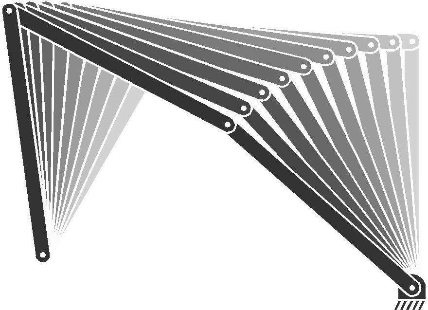
4 Inverse kinematics (IK) for a planar robot manipulator
By differentiating the forward kinematics function, a least norm inverse kinematics solution can be computed with
| \bm{\dot{\bm{x}}}=\bm{J}^{\dagger}\!(\bm{x})\;\bm{\dot{f}}, |
where the Jacobian \bm{J}(\bm{x}) corresponding to the end-effector forward kinematics function \bm{f}(\bm{x}) can be computed as (with a simplification for the orientation part by ignoring the manifold aspect)
| \displaystyle\bm{J} | \displaystyle=\begin{bmatrix}\textstyle-\sin(\bm{L}\bm{x})^{\scriptscriptstyle\top}\mathrm{diag}(\bm{\ell})\bm{L}\\ \textstyle\cos(\bm{L}\bm{x})^{\scriptscriptstyle\top}\mathrm{diag}(\bm{\ell})\bm{L}\\ \textstyle\bm{1}^{\scriptscriptstyle\top}\end{bmatrix} | ||
| \displaystyle=\begin{bmatrix}\textstyle J_{1,1}&J_{1,2}&J_{1,3}&\ldots\\ \textstyle J_{2,1}&J_{2,2}&J_{2,3}&\ldots\\ \textstyle J_{3,1}&J_{3,2}&J_{3,3}&\ldots\\ \end{bmatrix}\!\!, |
with
| \displaystyle J_{1,1}=-\ell_{1}\!\sin(x_{1})\!-\!\ell_{2}\!\sin(x_{1}\!+\!x_{2})\!-\!\ell_{3}\!\sin(x_{1}\!+\!x_{2}\!+\!x_{3})\!-\!\ldots,\quad | \displaystyle J_{1,2}=-\ell_{2}\!\sin(x_{1}\!+\!x_{2})\!-\!\ell_{3}\!\sin(x_{1}\!+\!x_{2}\!+\!x_{3})\!-\!\ldots,\quad | \displaystyle J_{1,3}=-\ell_{3}\!\sin(x_{1}\!+\!x_{2}\!+\!x_{3})\!-\!\ldots, | ||
| \displaystyle J_{2,1}=\ell_{1}\!\cos(x_{1})\!+\!\ell_{2}\!\cos(x_{1}\!+\!x_{2})\!+\!\ell_{3}\!\cos(x_{1}\!+\!x_{2}\!+\!x_{3})\!+\!\ldots, | \displaystyle J_{2,2}=\ell_{2}\!\cos(x_{1}\!+\!x_{2})\!+\!\ell_{3}\!\cos(x_{1}\!+\!x_{2}\!+\!x_{3})\!+\!\ldots, | \displaystyle J_{2,3}=\ell_{3}\!\cos(x_{1}\!+\!x_{2}\!+\!x_{3})\!+\!\ldots,\quad\ldots | ||
| \displaystyle J_{3,1}=1, | \displaystyle J_{3,2}=1, | \displaystyle J_{3,3}=1, |
In Python, this can be coded for the end-effector position part as
This Jacobian can be used to solve the inverse kinematics (IK) problem that consists of finding a robot pose to reach a target with the robot endeffector. The underlying optimization problem consists of minimizing a quadratic cost c=\|\bm{f}-\bm{\mu}\|^{2} , where \bm{f} is the position of the endeffector and \bm{\mu} is a target to reach with this endeffector. An optimization problem with a quadratic cost can be solved iteratively with a Gauss–Newton method, requiring to compute Jacobian pseudoinverses \bm{J}^{\dagger} , see Section 2.1 for details.
4.1 Numerical estimation of the Jacobian
Section 4 above presented an analytical solution for the Jacobian. A numerical solution can alternatively be estimated by computing
| J_{i,j}=\frac{\partial f_{i}(\bm{x})}{\partial x_{j}}\approx\frac{f_{i}(\bm{x}^{(j)})-f_{i}(\bm{x})}{\Delta}\quad\forall i,\forall j, |
with \bm{x}^{(j)} a vector of the same size as \bm{x} with elements
| x^{(j)}_{k}=\begin{cases}x_{k}+\Delta,&\text{if}\ k=j,\\ x_{k},&\text{otherwise},\end{cases} |
where \Delta is a small value for the approximation of the derivatives.
4.2 Inverse kinematics (IK) with task prioritization
In ( 14 ), the pseudoinverse provides a single least norm solution. This result can be generalized to obtain all solutions of the linear system with
| \bm{\dot{\bm{x}}}=\bm{J}^{\dagger}\!(\bm{x})\;\bm{\dot{f}}+\bm{N}\!(\bm{x})\;\bm{g}(\bm{x}), |
where \bm{g}(\bm{x}) is any desired gradient function and \bm{N}\!(\bm{x}) the nullspace projection operator
| \bm{N}\!(\bm{x})=\bm{I}-\bm{J}(\bm{x})^{\dagger}\bm{J}(\bm{x}). |
In the above, the solution is unique if and only if \bm{J}(\bm{x}) has full column rank, in which case \bm{N}(\bm{x}) is a zero matrix.
An alternative way of computing the nullspace projection matrix, numerically more robust, is to exploit the singular value decomposition
| \bm{J}^{\dagger}\!=\!\bm{U}\bm{\Sigma}\bm{V}^{\scriptscriptstyle\top}, |
to compute
| \bm{N}=\bm{\tilde{U}}\bm{\tilde{U}}^{\scriptscriptstyle\top}, |
where \bm{\tilde{U}} is a matrix formed by the columns of \bm{U} that span for the corresponding zero rows in \bm{\Sigma} .
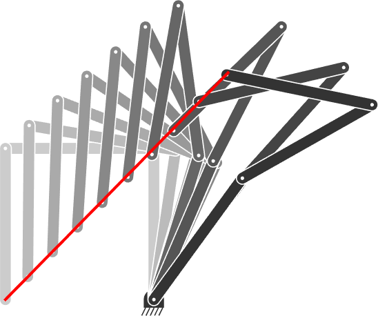
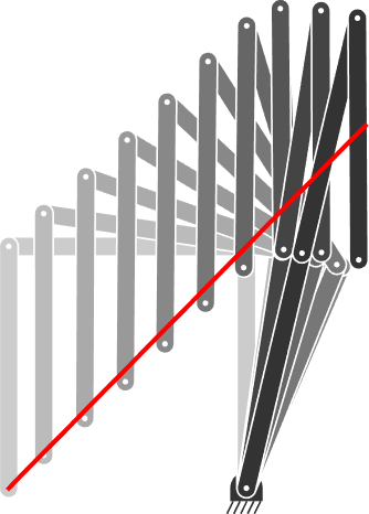
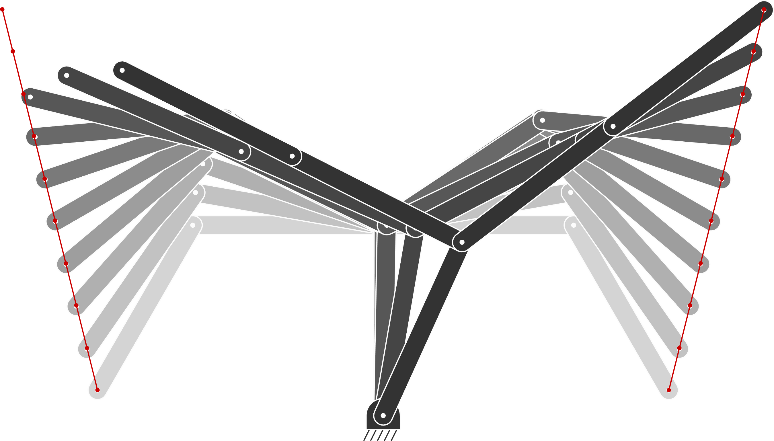
Figure 7 presents examples of nullspace controllers. Figure 6(a) shows a robot controller keeping its end-effector still as primary objective, while trying to move the first joint as secondary objective, which is achieved with the controller
| \bm{\dot{\bm{x}}}=\bm{J}^{\dagger}\!(\bm{x})\!\begin{bmatrix}0\\ 0\end{bmatrix}+\bm{N}\!(\bm{x})\!\begin{bmatrix}1\\ 0\\ 0\end{bmatrix}. |