5 Encoding with basis functions
Basis functions can be used to encode signals in a compact manner. It can be used to provide prior information about the encoded signals through a weighted superposition of basis functions acting as a dictionary of simpler signals that are combined to form more complex signals.
Basis functions can for example be used to encode trajectories, whose input is a 1D time variable and whose output can be multidimensional. For basis functions \bm{\phi}(t) described by a time or phase variable t , the corresponding continuous signal \bm{x}(t) is encoded with \bm{x}(t)=\bm{\phi}(t)\,\bm{w} , with t a continuous time variable and \bm{w} a vector containing the superposition weights. Basis functions can also be employed in a discretized form by providing a specific list of time steps, which is the form we will employ next.
The term movement primitive is often used in robotics to refer to the use of basis functions to encode trajectories. It corresponds to an organization of continuous motion signals in the form of a superposition in parallel and in series of simpler signals, which can be viewed as “building blocks” to create more complex movements, see Fig. 8 . This principle, coined in the context of motor control [ 9 ] , remains valid for a wide range of continuous time signals (for both analysis and synthesis).
The simpler form of movement primitives consists of encoding a movement as a weighted superposition of simpler movements. The compression aims at working in a subspace of reduced dimensionality, while denoising the signal and capturing the essential aspects of a movement.
5.1 Univariate trajectories
A univariate trajectory \bm{x}^{\text{\tiny 1D}}\in\mathbb{R}^{T} of T datapoints can be represented as a weighted sum of K basis functions with
| \bm{x}^{\text{\tiny 1D}}=\sum_{k=1}^{K}\bm{\phi}_{k}\;w^{\text{\tiny 1D}}_{k}=\bm{\phi}\;\bm{w}^{\text{\tiny 1D}}, |
where \bm{\phi} can be any set of basis functions, including some common forms that are presented below (see also [ 2 ] for more details).
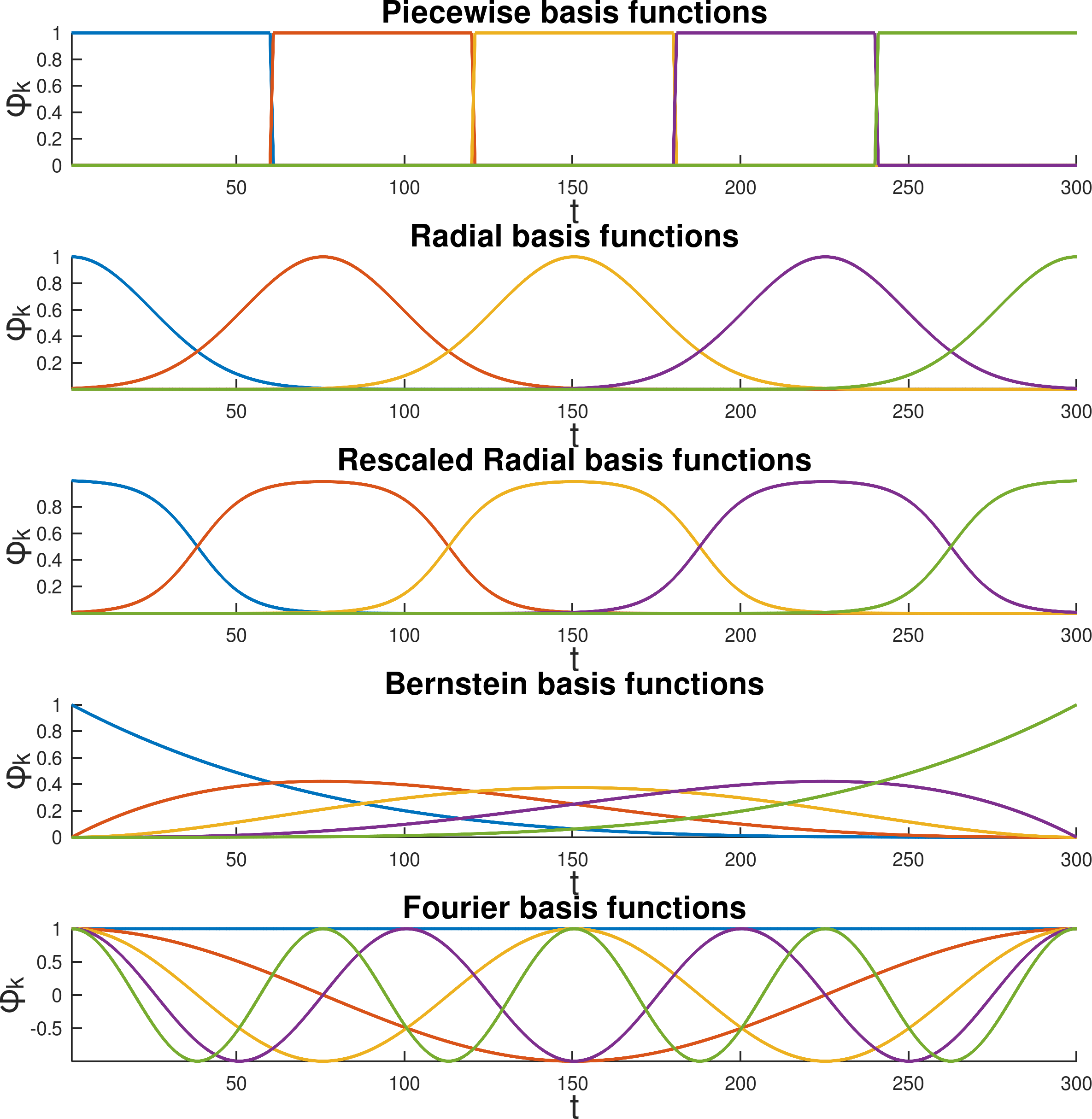
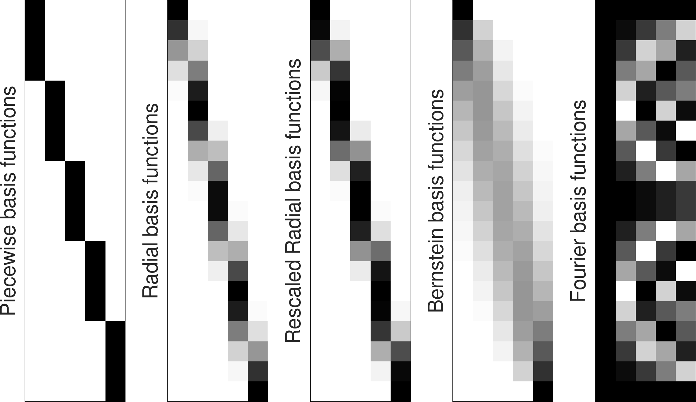
Piecewise constant basis functions
Piecewise constant basis functions can be computed in matrix form as
| \bm{\phi}=\bm{I}_{K}\otimes\bm{1}_{\frac{T}{K}}, |
where \bm{I}_{K} is an identity matrix of size K and \bm{1}_{\frac{T}{K}} is a vector of length \frac{T}{K} compose of unit elements, see Fig. 8 .
Radial basis functions (RBFs)
Gaussian radial basis functions (RBFs) can be computed in matrix form as
| \bm{\phi}=\exp(-\lambda\;\bm{E}\odot\bm{E}),\quad\text{with}\quad\bm{E}=\bm{t}\;\bm{1}_{K}^{\scriptscriptstyle\top}-\bm{1}_{T}\;{\bm{\mu}^{\text{\tiny s}}}^{\scriptscriptstyle\top}, |
where \lambda is bandwidth parameter, \odot is the elementwise (Hadamard) product operator, \bm{t}\in\mathbb{R}^{T} is a vector with entries linearly spaced between 0 to 1 , \bm{\mu}^{\text{\tiny s}}\in\mathbb{R}^{K} is a vector containing the RBF centers linearly spaced on the [0,1] range, and the \exp(\cdot) function is applied to each element of the matrix, see Fig. 8 .
RBFs can also be employed in a rescaled form by replacing each row \bm{\phi}_{k} with \frac{\bm{\phi}_{k}}{\sum_{i=1}^{K}\bm{\phi}_{i}} .
Bernstein basis functions
Bernstein basis functions (used for Bézier curves) can be computed as
| \bm{\phi}_{k}=\frac{(K-1)!}{(k-1)!(K-k)!}\;{(\bm{1}_{T}-\bm{t})}^{K-k}\;\odot\;\bm{t}^{k-1}, |
\forall k\in\{1,\ldots,K\} , where \bm{t}\in\mathbb{R}^{T} is a vector with entries linearly spaced between 0 to 1 , and (\cdot)^{d} is applied elementwise, see Fig. 8 .
Fourier basis functions
Fourier basis functions can be computed in matrix form as
| \bm{\phi}=\exp(\bm{t}\,\bm{\tilde{k}}^{\scriptscriptstyle\top}\,2\pi i), |
where the \exp(\cdot) function is applied to each element of the matrix, \bm{t}\in\mathbb{R}^{T} is a vector with entries linearly spaced between 0 to 1 , \bm{\tilde{k}}={[-K\!+\!1,-K\!+\!2,\ldots,K\!-\!2,K\!-\!1]}^{\scriptscriptstyle\top} , and i is the imaginary unit ( i^{2}=-1 ).
If \bm{x} is a real and even signal, the above formulation can be simplified to
| \bm{\phi}=\cos(\bm{t}\,\bm{k}^{\scriptscriptstyle\top}\,2\pi i), |
with \bm{k}={[0,1,\ldots,K\!-\!2,K\!-\!1]}^{\scriptscriptstyle\top} , see Fig. 8 .
Indeed, we first note that \exp(ai) is composed of a real part and an imaginary part with \exp(ai)=\cos(a)+i\sin(a) . We can see that for a given time step t , a real state x_{t} can be constructed with the Fourier series
| \displaystyle x_{t} | \displaystyle=\sum_{k=-K+1}^{K-1}w_{k}\exp(t\,k\,2\pi i) | ||
| \displaystyle=\sum_{k=-K+1}^{K-1}w_{k}\cos(t\,k\,2\pi) | |||
| \displaystyle=w_{0}+\sum_{k=1}^{K-1}2w_{k}\cos(t\,k\,2\pi), |
where we used the properties \cos(0)=1 and \cos(-a)=\cos(a) of the cosine function. Since we do not need direct correspondences between the Fourier transform and discrete cosine transform as in the above, we can omit the scaling factors for w_{k} and directly write the decomposition as in ( 21 ).
5.2 Multivariate trajectories
A multivariate trajectory \bm{x}\in\mathbb{R}^{DT} of T datapoints of dimension D can similarly be computed as
| \bm{x}=\sum_{k=1}^{K}\bm{\Psi}_{k}\;w_{k}=\bm{\Psi}\;\bm{w},\quad\text{with}\quad\bm{\Psi}=\bm{\phi}\otimes\bm{I}=\left[\begin{matrix}\bm{I}\phi_{1,1}&\bm{I}\phi_{2,1}&\cdots&\bm{I}\phi_{K,1}\\ \bm{I}\phi_{1,2}&\bm{I}\phi_{2,2}&\cdots&\bm{I}\phi_{K,2}\\ \vdots&\vdots&\ddots&\vdots\\ \bm{I}\phi_{1,T}&\bm{I}\phi_{2,T}&\cdots&\bm{I}\phi_{K,T}\end{matrix}\right], |
where \otimes the Kronecker product operator and \bm{I} is an identity matrix of size D\times D .
In the above, \bm{I} can alternatively be replaced by a rectangular matrix \bm{S} acting as a coordination matrix.
5.3 Multidimensional inputs
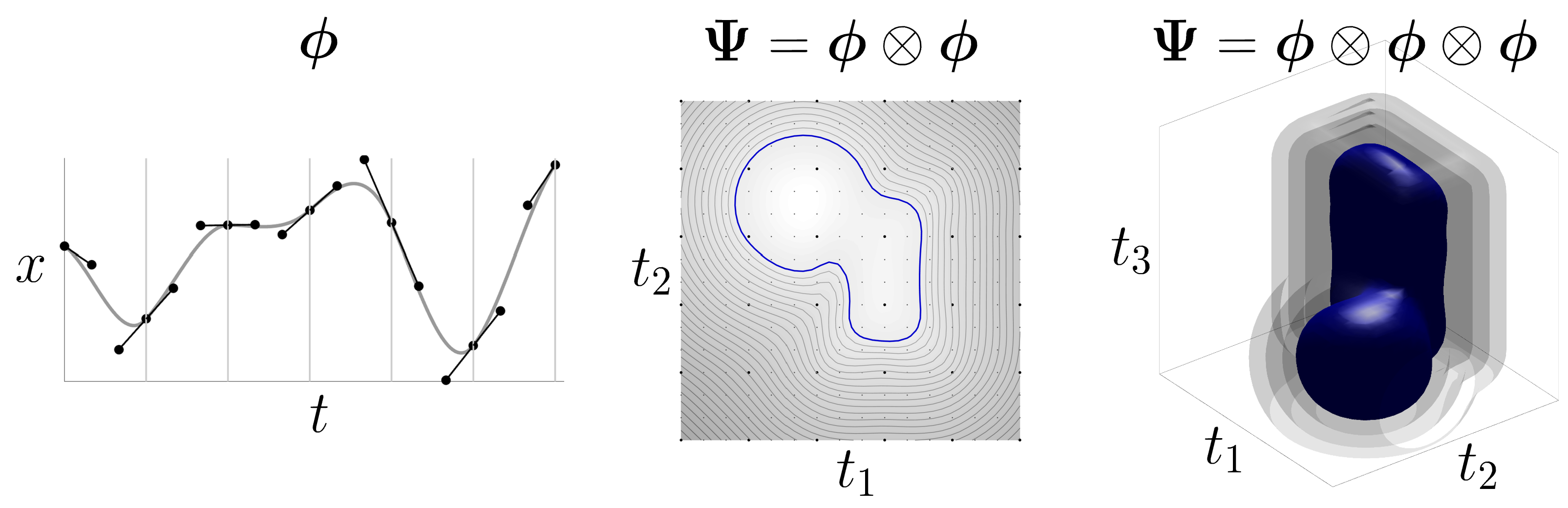
Basis functions can also be used to encode signals generated by multivariate inputs t_{i} . For example, a Bézier surface uses two input variables t_{1} and t_{2} to cover a spatial range and generates an output variable describing the height of the surface within this rectangular region. This surface (represented as a colormap in Fig. 9 - center ) can be constructed from a 1D input signal by leveraging the Kronecker product operation, namely
| \bm{\Psi}=\bm{\phi}\,\otimes\,\bm{\phi} |
in matrix form, or
| \bm{\Psi}(\bm{t})=\bm{\phi}(t_{1})\,\otimes\,\bm{\phi}(t_{2}) |
in analytic form.
When using splines of the form \bm{\phi}=\bm{T}\bm{B}\bm{C} , ( 24 ) can equivalently be computed as
| \bm{\Psi}(\bm{t})=\big(\bm{T}(t_{1})\,\otimes\,\bm{T}(t_{2})\big)\,\big(\bm{B}\bm{C}\,\otimes\,\bm{B}\bm{C}\big), |
which means that \big(\bm{B}\bm{C}\,\otimes\,\bm{B}\bm{C}\big) can be precomputed.
As for the unidimensional version, we still maintain a linear reconstruction \bm{x}=\bm{\Psi}\,\bm{w} , where \bm{x} and \bm{w} are vectorized versions of surface heights and superposition weights, which can be reorganized as 2D arrays if required.
Successive Kronecker products can be used so that any number of input and output dimensions {d^{\text{\tiny in}}} and {d^{\text{\tiny out}}} can be considered, with
| \bm{\Psi}=\underbrace{\bm{\phi}\,\otimes\,\bm{\phi}\,\otimes\cdots\otimes\,\bm{\phi}}_{d^{\text{\tiny in}}}\,\otimes\,\bm{I}_{d^{\text{\tiny out}}}. |
For example, a vector field in 3D can be encoded with basis functions
| \bm{\Psi}=\bm{\phi}\,\otimes\,\bm{\phi}\,\otimes\,\bm{\phi}\,\otimes\,\bm{I}_{3}, |
where \bm{I}_{3} is a 3\!\times\!3 identity matrix to encode the 3 elements of the vector.
Figure 9 shows examples with various input dimensions. In Fig. 9 - center , several equidistant contours are displayed as closed paths, with the one corresponding to the object contour (distance zero) represented in blue. In Fig. 9 - left , several isosurfaces are displayed as 3D shapes, with the one corresponding to the object surface (distance zero) represented in blue. The algorithm used to determine the closed contours (in 2D) and isosurfaces (in 3D) is exploited here for visualization purpose, but can also be exploited if an explicit definition of shapes is required (instead of an implicit surface representation).
The analytic expression provided by the proposed encoding can also be used to express the derivatives as analytic expressions. This can be used for control and planning problem, such as moving closer or away from objects, or orienting the robot gripper to be locally aligned with the surface of an object.
5.4 Derivatives
By using basis functions as analytic expressions, the derivatives are easy to compute. For example, for 2D inputs as in ( 24 ), we have
| \frac{\partial\bm{\Psi}(\bm{t})}{\partial t_{1}}=\frac{\partial\bm{\phi}(t_{1})}{\partial t_{1}}\,\otimes\,\bm{\phi}(t_{2}),\qquad\qquad\frac{\partial\bm{\Psi}(\bm{t})}{\partial t_{2}}=\bm{\phi}(t_{1})\,\otimes\,\frac{\partial\bm{\phi}(t_{2})}{\partial t_{2}}. |
By modeling a signed distance function as x=f(\bm{t}) , the derivatives can for example be used to find a point on the contour (with distance zero). Such problem can be solved with Gauss–Newton optimization with the cost c(\bm{t})=\frac{1}{2}f(\bm{t})^{2} , by starting from an initial guess \bm{t}_{0} . In the above example, the Jacobian is then given by
| \bm{J}(\bm{t})=\begin{bmatrix}\frac{\partial\bm{\Psi}(\bm{t})}{\partial t_{1}}\,\bm{w}\\[5.690551pt] \frac{\partial\bm{\Psi}(\bm{t})}{\partial t_{2}}\,\bm{w}\end{bmatrix}, |
and the update can be computed recursively with
| \bm{t}_{k+1}\;\leftarrow\;\bm{t}_{k}-\bm{J}(\bm{t}_{k})^{\dagger}f(\bm{t}_{k}), |
as in Equation ( 8 ), where \bm{J}(\bm{t}_{k})^{\scriptscriptstyle\top}f(\bm{t}_{k}) is a gradient and \bm{J}(\bm{t}_{k})^{\scriptscriptstyle\top}\bm{J}(\bm{t}_{k}) a Hessian matrix.
For two shapes encoded as SDFs f_{1}(\bm{t}_{1}) and f_{2}(\bm{t}_{2}) using basis functions, finding the shortest segment between the two shapes boils down to the Gauss–Newton optimization of a pair of points \bm{t}_{1} and \bm{t}_{2} organized as \bm{t}=\begin{bmatrix}\bm{t}_{1}\\ \bm{t}_{2}\end{bmatrix} with the cost
| c(\bm{t})=\frac{1}{2}\,f_{1}(\bm{t}_{1})^{2}+\frac{1}{2}\,f_{2}(\bm{t}_{2})^{2}+\frac{1}{2}\,\|\bm{A}\,\bm{t}_{2}-\bm{t}_{1}+\bm{b}\|^{2}, |
which is composed of quadratic residual terms, where \bm{A} and \bm{b} are the rotation matrix and translation vector offset between the two objects, respectively. The Jacobian of the above cost is given by
| \bm{J}(\bm{t})=\begin{bmatrix}\bm{J}_{1}(\bm{t}_{1})&\bm{0}\\ \bm{0}&\bm{J}_{2}(\bm{t}_{2})\\ -\bm{I}&\bm{A}\end{bmatrix}, |
where \bm{J}_{1}(\bm{t}_{1}) and \bm{J}_{2}(\bm{t}_{2}) are the derivatives of the two SDFs as given by ( 29 ).
Similarly to ( 30 ), the Gauss–Newton update step is then given by
| \bm{t}_{k+1}\;\leftarrow\;\bm{t}_{k}-\bm{J}(\bm{t}_{k})^{\dagger}\begin{bmatrix}f_{1}(\bm{t}_{1,k})\\ f_{2}(\bm{t}_{2,k})\\ \bm{A}\,\bm{t}_{2,k}-\bm{t}_{1,k}+\bm{b}\end{bmatrix}. |
A prioritized optimization scheme can also be used to have the two points on the shape boundaries as primary objective and to move these points closer as secondary objective, with a corresponding Gauss–Newton update step given by
| \displaystyle\bm{t}_{k+1} | \displaystyle\leftarrow\;\bm{t}_{k}-\bm{J}_{12}^{\dagger}\begin{bmatrix}\textstyle f_{1}(\bm{t}_{1,k})\\ \textstyle f_{2}(\bm{t}_{2,k})\end{bmatrix}+\bm{N}_{12}\;\bm{J}_{3}^{\dagger}\;(\bm{A}\,\bm{t}_{2,k}-\bm{t}_{1,k}+\bm{b}), | ||
| \displaystyle\text{where}\quad\bm{J}_{12} | \displaystyle=\begin{bmatrix}\textstyle\bm{J}_{1}(\bm{t}_{1})&\bm{0}\\ \textstyle\bm{0}&\bm{J}_{2}(\bm{t}_{2})\end{bmatrix},\quad\bm{N}_{12}=\bm{I}-\bm{J}_{12}^{\dagger}\bm{J}_{12},\quad\bm{J}_{3}=\begin{bmatrix}\textstyle-\bm{I}&\bm{A}\end{bmatrix}. |
5.5 Concatenated basis functions
When encoding entire signals, some dictionaries such as Bernstein basis functions require to set polynomials of high order to encode long or complex signals. Instead of considering a global encoding, it can be useful to split the problem as a set of local fitting problems which can consider low order polynomials. A typical example is the encoding of complex curves as a concatenation of simple Bézier curves. When concatenating curves, constraints on the superposition weights are typically considered. These weights can be represented as control points in the case of Bézier curves and splines. We typically constrain the last point of a curve and the first point of the next curve to maintain the continuity of the curve. We also typically constrain the control points before and after this joint to be symmetric, effectively imposing smoothness.
In practice, this can be achieved efficiently by simply replacing \bm{\phi} with \bm{\phi}\bm{C} in the above equations, where \bm{C} is a tall rectangular matrix. This further reduces the number of superposition weights required in the encoding, as the constraints also reduce the number of free variables.
For example, for the concatenation of Bézier curves, we can define \bm{C} as
| \bm{C}=\begin{bmatrix}1&0&\cdots&0&0&\cdots\\ 0&1&\cdots&0&0&\cdots\\ \vdots&\vdots&\ddots&\vdots&\vdots&\ddots\\ 0&0&\cdots&1&0&\cdots\\ 0&0&\cdots&0&1&\cdots\\ 0&0&\cdots&0&1&\cdots\\ 0&0&\cdots&-1&2&\cdots\\ \vdots&\vdots&\ddots&\vdots&\vdots&\ddots\end{bmatrix}, |
where the pattern \begin{bmatrix}1&0\\ 0&1\\ 0&1\\ -1&2\end{bmatrix} is repeated for each junction of two consecutive Bézier curves. For two concatenated cubic Bézier curves, each composed of 4 Bernstein basis functions, we can see locally that this operator yields a constraint of the form
| \begin{bmatrix}w_{3}\\ w_{4}\\ w_{5}\\ w_{6}\end{bmatrix}=\begin{bmatrix}1&0\\ 0&1\\ 0&1\\ -1&2\end{bmatrix}\begin{bmatrix}a\\ b\end{bmatrix}, |
which ensures that w_{4}=w_{5} and w_{6}=-w_{3}+2w_{5} . These constraints guarantee that the last control point and the first control point of the next segment are the same, and that the control point before and after are symmetric with respect to this junction point, see Fig. 9 - left .
5.6 Batch computation of basis functions coefficients
Based on observed data \bm{x} , the superposition weights \bm{w} can be estimated as a simple least squares estimate
| \bm{w}=\bm{\Psi}^{\dagger}\bm{x}, |
or as the regularized version (ridge regression)
| \bm{w}={(\bm{\Psi}^{\scriptscriptstyle\top}\bm{\Psi}+\lambda\bm{I})}^{-1}\bm{\Psi}^{\scriptscriptstyle\top}\bm{x}. |
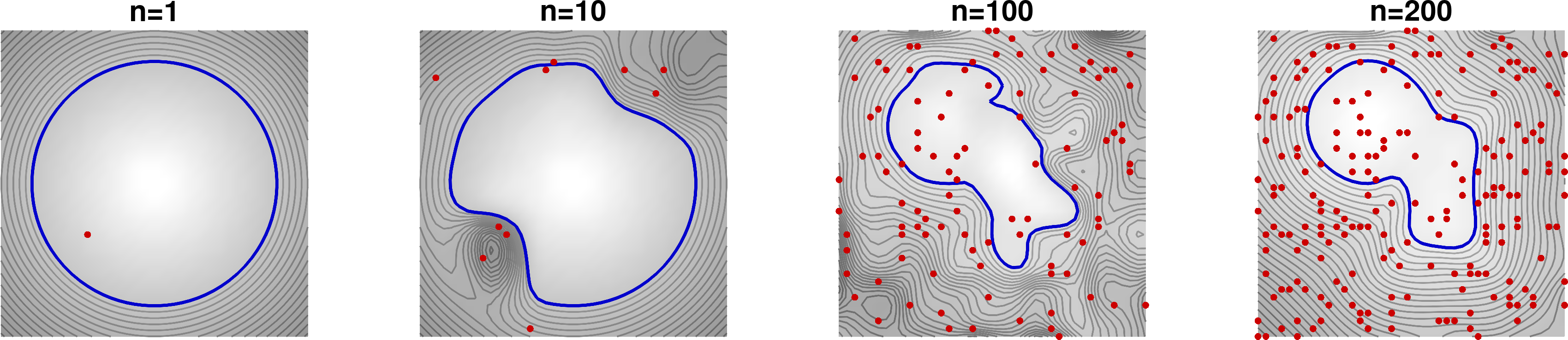
5.7 Recursive computation of basis functions coefficients
The same result can be obtained by recursive computation, by providing the datapoints one-by-one or by groups of points. The algorithm starts from an initial estimate of \bm{w} that is iteratively refined with the arrival of new datapoints, see Fig. 10 .
This recursive least squares algorithm exploits the Sherman-Morrison-Woodbury formulas that relate the inverse of a matrix after a small-rank perturbation to the inverse of the original matrix, namely
| \left(\bm{B}+\bm{U}\bm{V}\right)^{-1}=\bm{B}^{-1}-\overbrace{\bm{B}^{-1}\bm{U}\left(\bm{I}+\bm{V}\bm{B}^{-1}\bm{U}\right)^{-1}\bm{V}\bm{B}^{-1}}^{\bm{E}} |
with \bm{U}\!\in\!\mathbb{R}^{n\times m} and \bm{V}\!\in\!\mathbb{R}^{m\times n} . When m\!\ll\!n , the correction term \bm{E} can be computed more efficiently than inverting \bm{B}+\bm{U}\bm{V} .
By defining \bm{B}\!=\!\bm{\Psi}^{\scriptscriptstyle\top}\bm{\Psi} , the above relation can be exploited to update the least squares solution ( 44 ) when new datapoints become available. Indeed, if \bm{\Psi}_{\!\scriptscriptstyle\mathrm{new}}=\begin{bmatrix}\bm{\Psi},\bm{V}\end{bmatrix} and \bm{x}_{\!\scriptscriptstyle\mathrm{new}}=\begin{bmatrix}\bm{x}\\ \bm{v}\end{bmatrix} , we can see that
| \displaystyle\bm{B}_{\!\scriptscriptstyle\mathrm{new}} | \displaystyle=\bm{\Psi}_{\!\scriptscriptstyle\mathrm{new}}^{\scriptscriptstyle\top}\bm{\Psi}_{\!\scriptscriptstyle\mathrm{new}} | ||
| \displaystyle=\bm{\Psi}^{\scriptscriptstyle\top}\bm{\Psi}+\bm{V}^{\scriptscriptstyle\top}\bm{V} | |||
| \displaystyle=\bm{B}+\bm{V}^{\scriptscriptstyle\top}\bm{V}, |
whose inverse can be computed using ( 45 ), yielding
| \bm{B}_{\!\scriptscriptstyle\mathrm{new}}^{-1}=\bm{B}^{-1}-\underbrace{\bm{B}^{-1}\bm{V}^{\scriptscriptstyle\top}\left(\bm{I}+\bm{V}\bm{B}^{-1}\bm{V}^{\scriptscriptstyle\top}\right)^{-1}}_{\bm{K}}\bm{V}\bm{B}^{-1}. |
This is exploited to estimate the update as
| \bm{w}_{\!\scriptscriptstyle\mathrm{new}}=\bm{w}+\bm{K}\Big(\bm{v}-\bm{V}\bm{w}\Big), |
with Kalman gain
| \bm{K}=\bm{B}^{-1}\bm{V}^{\scriptscriptstyle\top}\left(\bm{I}+\bm{V}\bm{B}^{-1}\bm{V}^{\scriptscriptstyle\top}\right)^{-1}. |
The above equations can be used recursively, with \bm{B}_{\!\scriptscriptstyle\mathrm{new}}^{-1} and \bm{w}_{\!\scriptscriptstyle\mathrm{new}} the updates that will become \bm{B}^{-1} and \bm{w} for the next iteration. Note that the above iterative computation only uses \bm{B}^{-1} , which is the variable stored in memory. Namely, we never use \bm{B} , only the inverse. For recursive ridge regression, the algorithm starts with \bm{B}^{-1}=\frac{1}{\lambda}\bm{I} . After all datapoints are used, the estimate of \bm{w} is exactly the same as the ridge regression result ( 44 ) computed in batch form. Algorithm 1 summarizes the computation steps.