6 Linear quadratic tracking (LQT)
Linear quadratic tracking (LQT) is a simple form of optimal control that trades off tracking and control costs expressed as quadratic terms over a time horizon, with the evolution of the state described in a linear form. The LQT problem is formulated as the minimization of the cost
| \displaystyle c | \displaystyle={\big(\bm{\mu}_{T}\!-\!\bm{x}_{T}\big)}^{\scriptscriptstyle\top}\bm{Q}_{T}\big(\bm{\mu}_{T}\!-\!\bm{x}_{T}\big)+\sum_{t=1}^{T-1}\Big({\big(\bm{\mu}_{t}\!-\!\bm{x}_{t}\big)}^{\scriptscriptstyle\top}\bm{Q}_{t}\big(\bm{\mu}_{t}\!-\!\bm{x}_{t}\big)\;+\;\bm{u}_{t}^{\scriptscriptstyle\top}\bm{R}_{t}\;\bm{u}_{t}\Big) | ||
| \displaystyle={\big(\bm{\mu}-\bm{x}\big)}^{\scriptscriptstyle\top}\bm{Q}\big(\bm{\mu}-\bm{x}\big)\;+\;\bm{u}^{\scriptscriptstyle\top}\!\bm{R}\bm{u}, |
with \bm{x}\!=\!{\begin{bmatrix}\bm{x}_{1}^{\scriptscriptstyle\top},\bm{x}_{2}^{\scriptscriptstyle\top},\ldots,\bm{x}_{T}^{\scriptscriptstyle\top}\end{bmatrix}}^{\scriptscriptstyle\top} the evolution of the state variables, \bm{u}\!=\!{\begin{bmatrix}\bm{u}_{1}^{\scriptscriptstyle\top},\bm{u}_{2}^{\scriptscriptstyle\top},\ldots,\bm{u}_{T-1}^{\scriptscriptstyle\top}\end{bmatrix}}^{\scriptscriptstyle\top} the evolution of the control commands, and \bm{\mu}\!=\!{\begin{bmatrix}\bm{\mu}_{1}^{\scriptscriptstyle\top},\bm{\mu}_{2}^{\scriptscriptstyle\top},\ldots,\bm{\mu}_{T}^{\scriptscriptstyle\top}\end{bmatrix}}^{\scriptscriptstyle\top} the evolution of the tracking targets. \bm{Q}\!=\!\mathrm{blockdiag}(\bm{Q}_{1},\bm{Q}_{2},\ldots,\bm{Q}_{T}) represents the evolution of the precision matrices \bm{Q}_{t} , and \bm{R}\!=\!\mathrm{blockdiag}(\bm{R}_{1},\bm{R}_{2},\ldots,\bm{R}_{T-1}) represents the evolution of the control weight matrices \bm{R}_{t} .
The evolution of the system is linear, described by
| \bm{x}_{t+1}=\bm{A}_{t}\bm{x}_{t}+\bm{B}_{t}\bm{u}_{t}, |
yielding at trajectory level
| \bm{x}=\bm{S}_{\bm{x}}\bm{x}_{1}+\bm{S}_{\bm{u}}\bm{u}, |
see Appendix A for details.
With open loop control commands organized as a vector \bm{u} , the solution of ( 52 ) subject to \bm{x}=\bm{S}_{\bm{x}}\bm{x}_{1}+\bm{S}_{\bm{u}}\bm{u} is analytic, given by
| \bm{\hat{u}}={\big(\bm{S}_{\bm{u}}^{\scriptscriptstyle\top}\bm{Q}\bm{S}_{\bm{u}}+\bm{R}\big)}^{-1}\bm{S}_{\bm{u}}^{\scriptscriptstyle\top}\bm{Q}\big(\bm{\mu}-\bm{S}_{\bm{x}}\bm{x}_{1}\big). |
The residuals of this least squares solution provides information about the uncertainty of this estimate, in the form of a full covariance matrix (at control trajectory level)
| \bm{\hat{\Sigma}}^{\bm{u}}={\big(\bm{S}_{\bm{u}}^{\scriptscriptstyle\top}\bm{Q}\bm{S}_{\bm{u}}+\bm{R}\big)}^{-1}, |
which provides a probabilistic interpretation of LQT.
The batch computation approach facilitates the creation of bridges between learning and control. For example, in learning from demonstration, the observed (co)variations in a task can be formulated as an LQT objective function, which then provides a trajectory distribution in control space that can be converted to a trajectory distribution in state space. All the operations are analytic and only exploit basic linear algebra.
The approach can also be extended to model predictive control (MPC), iterative LQR (iLQR) and differential dynamic programming (DDP), whose solution needs this time to be interpreted locally at each iteration step of the algorithm, as we will see later in the technical report.
Example: Bimanual tennis serve
LQT can be used to solve a ballistic task mimicking a bimanual tennis serve problem. In this problem, a ball is thrown by one hand and then hit by the other, with the goal of bringing the ball to a desired target, see Fig. 11 . The problem is formulated as in ( 52 ), namely
| \min_{\bm{u}}{(\bm{\mu}-\bm{x})}^{\!{\scriptscriptstyle\top}}\bm{Q}(\bm{\mu}-\bm{x})\;+\;\bm{u}^{\!{\scriptscriptstyle\top}}\!\bm{R}\bm{u},\;\text{s.t.}\;\bm{x}=\bm{S}_{\bm{x}}\bm{x}_{1}+\bm{S}_{\bm{u}}\bm{u}, |
where \bm{x} represents the state trajectory of the 3 agents (left hand, right hand and ball), where only the hands can be controlled by a series of acceleration commands \bm{u} that can be estimated by LQT.
In the above problem, \bm{Q} is a precision matrix and \bm{\mu} is a reference vector describing at specific time steps the targets that the three agents must reach. The linear systems are described according to the different phases of the task, see Appendix C for details. As shown above, the constrained objective in ( 57 ) can be solved by least squares, providing an analytical solution given by ( 55 ), see also Fig. 11 for the visualization of the result for a given target and for given initial poses of the hands.
6.1 LQT with smoothness cost
Linear quadratic tracking (LQT) can be used with dynamical systems described as simple integrators. With single integrators, the states correspond to positions, with velocity control commands. With double integrators, the states correspond to positions and velocities, with acceleration control commands. With triple integrators, the states correspond to positions, velocities and accelerations, with jerk control commands, etc.
Figure 12 shows an example of LQT for a task that consist of passing through a set of viapoints. The left and right graphs show the result for single and double integrators, respectively. The graph in the center also considers a single integrator, by redefining the weight matrix \bm{R} of the control cost to ensure smoothness. This can be done by replacing the standard diagonal \bm{R} matrix in ( 52 ) with
| \bm{R}=\left[\begin{matrix}2&-1&0&0&\cdots&0&0\\ -1&2&-1&0&\cdots&0&0\\ 0&-1&2&-1&\cdots&0&0\\ \vdots&\vdots&\vdots&\vdots&\ddots&\vdots&\vdots\\ 0&0&0&0&\cdots&2&-1\\ 0&0&0&0&\cdots&-1&2\end{matrix}\right]\otimes\bm{I}_{D}. |
6.2 LQT with control primitives
If we assume that the control commands profile \bm{u} is composed of control primitives (CP) with \bm{u}=\bm{\Psi}\bm{w} , the objective becomes
| \min_{\bm{w}}{(\bm{x}-\bm{\mu})}^{\!{\scriptscriptstyle\top}}\bm{Q}(\bm{x}-\bm{\mu})\;+\;\bm{w}^{\!{\scriptscriptstyle\top}}\bm{\Psi}^{\!{\scriptscriptstyle\top}}\bm{R}\bm{\Psi}\bm{w},\quad\text{s.t.}\quad\bm{x}=\bm{S}_{\bm{x}}\bm{x}_{1}+\bm{S}_{\bm{u}}\bm{\Psi}\bm{w}, |
with a solution given by
| \bm{\hat{w}}={\big(\bm{\Psi}^{\!{\scriptscriptstyle\top}}\bm{S}_{\bm{u}}^{\scriptscriptstyle\top}\bm{Q}\bm{S}_{\bm{u}}\bm{\Psi}+\bm{\Psi}^{\!{\scriptscriptstyle\top}}\bm{R}\bm{\Psi}\big)}^{-1}\bm{\Psi}^{\!{\scriptscriptstyle\top}}\bm{S}_{\bm{u}}^{\scriptscriptstyle\top}\bm{Q}\big(\bm{\mu}-\bm{S}_{\bm{x}}\bm{x}_{1}\big), |
which is used to compute the trajectory \bm{\hat{u}}=\bm{\Psi}\bm{\hat{w}} in control space, corresponding to the list of control commands organized in vector form. Similarly to ( 56 ), the residuals of the least squares solution provides a probabilistic approach to LQT with control primitives. Note also that the trajectory in control space can be converted to a trajectory in state space with \bm{\hat{x}}=\bm{S}_{\bm{x}}\bm{x}_{1}+\bm{S}_{\bm{u}}\bm{\hat{u}} . Thus, since all operations are linear, a covariance matrix on \bm{w} can be converted to a covariance on \bm{u} and on \bm{x} . A similar linear transformation is used in the context of probabilistic movement primitives (ProMP) [ 12 ] to map a covariance matrix on \bm{w} to a covariance on \bm{x} . LQT with control primitives provides a more general approach by considering both control and state spaces. It also has the advantage of reframing the method to the more general context of optimal control, thus providing various extension opportunities.
Several forms of basis functions can be considered, including stepwise control commands, radial basis functions (RBFs), Bernstein polynomials, Fourier series, or learned basis functions, which are organized as a dictionary matrix \bm{\Psi} . Dictionaries for multivariate control commands can be generated with a Kronecker product operator \otimes as
| \bm{\Psi}=\bm{\phi}\otimes\bm{C}, |
where the matrix \bm{\phi} is a horizontal concatenation of univariate basis functions, and \bm{C} is a coordination matrix, which can be set to an identity matrix \bm{I}_{D} for the generic case of control variables with independent basis functions for each dimension d\in\{1,\ldots,D\} .
Note also that in some situations, \bm{R} can be set to zero because the regularization role of \bm{R} in the original problem formulation can sometimes be redundant with the use of sparse basis functions.
6.3 LQR with a recursive formulation
The LQR problem is formulated as the minimization of the cost
| c(\bm{x}_{1},\bm{u})=c_{T}(\bm{x}_{T})+\sum_{t=1}^{T-1}c_{t}(\bm{x}_{t},\bm{u}_{t})\;=\bm{x}_{T}^{\scriptscriptstyle\top}\bm{Q}_{T}\bm{x}_{T}+\sum_{t=1}^{T-1}\Big(\bm{x}_{t}^{\scriptscriptstyle\top}\bm{Q}_{t}\bm{x}_{t}+\bm{u}_{t}^{\scriptscriptstyle\top}\bm{R}_{t}\,\bm{u}_{t}\Big),\quad\text{s.t.}\quad\bm{x}_{t+1}=\bm{A}_{t}\bm{x}_{t}+\bm{B}_{t}\bm{u}_{t}, |
where c without index refers to the total cost (cumulative cost). We also define the partial cumulative cost
| v_{t}(\bm{x}_{t},\bm{u}_{t:T-1})=c_{T}(\bm{x}_{T})+\sum_{s=t}^{T-1}c_{s}(\bm{x}_{t},\bm{u}_{t}), |
which depends on the states and control commands, except for v_{T} that only depends on the state.
We define the value function as the value taken by v_{t} when applying optimal control commands, namely
| \hat{v}_{t}(\bm{x}_{t})=\min_{\bm{u}_{t:T-1}}v_{t}(\bm{x}_{t},\bm{u}_{t:T-1}). |
We will use the dynamic programming principle to reduce the minimization in ( 61 ) over the entire sequence of control commands \bm{u}_{t:T-1} to a sequence of minimization problems over control commands at a single time step, by proceeding backwards in time.
By inserting ( 60 ) in ( 61 ), we observe that
| \displaystyle\hat{v}_{t}(\bm{x}_{t}) | \displaystyle=\min_{\bm{u}_{t:T-1}}\Big(c_{T}(\bm{x}_{T})+\sum_{s=t}^{T-1}c_{s}(\bm{x}_{t},\bm{u}_{t})\Big) | ||
| \displaystyle=\min_{\bm{u}_{t}}c_{t}(\bm{x}_{t},\bm{u}_{t})\!+\!\!\!\min_{\bm{u}_{t+1:T-1}}\!\!\!\Big(\!c_{T}(\bm{x}_{T})\!+\!\!\sum_{s=t+1}^{T-1}\!\!c_{s}(\bm{x}_{t},\bm{u}_{t})\!\Big) | |||
| \displaystyle=\min_{\bm{u}_{t}}\underbrace{c_{t}(\bm{x}_{t},\bm{u}_{t})+\hat{v}_{t+1}(\bm{x}_{t+1})}_{q_{t}(\bm{x}_{t},\bm{u}_{t})}, |
where q_{t} is called the q-function .
By starting from the last time step T , and by relabeling \bm{Q}_{T} as \bm{V}_{T} , we can see that \hat{v}_{T}(\bm{x}_{T})=c_{T}(\bm{x}_{T}) is independent of the control commands, taking the quadratic error form
| \hat{v}_{T}=\bm{x}_{T}^{\scriptscriptstyle\top}\bm{V}_{T}\bm{x}_{T}, |
which only involves the final state \bm{x}_{T} . We will show that \hat{v}_{T-1} has the same quadratic form as \hat{v}_{T} , enabling the backward recursive computation of \hat{v}_{t} from t=T-1 to t=1 .
With ( 62 ), the dynamic programming recursion takes the form
| \hat{v}_{t}=\min_{\bm{u}_{t}}\begin{bmatrix}\bm{x}_{t}\\ \bm{u}_{t}\end{bmatrix}^{\scriptscriptstyle\top}\begin{bmatrix}\bm{Q}_{t}&\bm{0}\\ \bm{0}&\bm{R}_{t}\end{bmatrix}\begin{bmatrix}\bm{x}_{t}\\ \bm{u}_{t}\end{bmatrix}+\bm{x}_{t+1}^{\scriptscriptstyle\top}\bm{V}_{t+1}\bm{x}_{t+1}. |
By substituting \bm{x}_{{t+1}}=\bm{A}_{t}\bm{x}_{t}+\bm{B}_{t}\bm{u}_{t} into ( 64 ), \hat{v}_{t} can be rewritten as
| \hat{v}_{t}=\min_{\bm{u}_{t}}\begin{bmatrix}\bm{x}_{t}\\ \bm{u}_{t}\end{bmatrix}^{\scriptscriptstyle\top}\begin{bmatrix}\bm{Q}_{\bm{x}\bm{x},t}&\bm{Q}_{\bm{u}\bm{x},t}^{\scriptscriptstyle\top}\\ \bm{Q}_{\bm{u}\bm{x},t}&\bm{Q}_{\bm{u}\bm{u},t}\end{bmatrix}\begin{bmatrix}\bm{x}_{t}\\ \bm{u}_{t}\end{bmatrix},\quad\text{where}\quad\left\{\begin{aligned} \bm{Q}_{\bm{x}\bm{x},t}&=\bm{A}_{t}^{\scriptscriptstyle\top}\bm{V}_{t+1}\bm{A}_{t}+\bm{Q}_{t},\\ \bm{Q}_{\bm{u}\bm{u},t}&=\bm{B}_{t}^{\scriptscriptstyle\top}\bm{V}_{t+1}\bm{B}_{t}+\bm{R}_{t},\\ \bm{Q}_{\bm{u}\bm{x},t}&=\bm{B}_{t}^{\scriptscriptstyle\top}\bm{V}_{t+1}\bm{A}_{t}.\end{aligned}\right. |
An optimal control command \bm{\hat{u}}_{t} can be computed by differentiating ( 65 ) with respect to \bm{u}_{t} and equating to zero, providing a feedback law
| \bm{\hat{u}}_{t}=-\bm{K}_{t}\,\bm{x}_{t},\quad\text{with}\quad\bm{K}_{t}=\bm{Q}_{\bm{u}\bm{u},t}^{-1}\,\bm{Q}_{\bm{u}\bm{x},t}. |
By introducing ( 66 ) back into ( 65 ), the resulting value function \hat{v}_{t} has the quadratic form
| \hat{v}_{t}=\bm{x}_{t}^{\scriptscriptstyle\top}\bm{V}_{t}\bm{x}_{t},\quad\text{with}\quad\bm{V}_{t}=\bm{Q}_{\bm{x}\bm{x},t}-\bm{Q}_{\bm{u}\bm{x},t}^{\scriptscriptstyle\top}\,\bm{Q}_{\bm{u}\bm{u},t}^{-1}\,\bm{Q}_{\bm{u}\bm{x},t}. |
We observe that ( 67 ) has the same quadratic form as ( 63 ), so that ( 62 ) can be solved recursively. We thus obtain a backward recursion procedure in which \bm{V}_{t} is evaluated recursively from t=T-1 to t=1 , starting from \bm{V}_{T}=\bm{Q}_{T} , which corresponds to a Riccati equation.
After all feedback gain matrices \bm{K}_{t} have been computed by backward recursion, a forward recursion can be used to compute the evolution of the state, starting from \bm{x}_{1} , by using the linear system \bm{x}_{t+1}=\bm{A}_{t}\bm{x}_{t}+\bm{B}_{t}\bm{u}_{t} and the control policy \bm{u}_{t}=-\bm{K}_{t}\bm{x}_{t} , see Algorithm 2 for the summary of the overall procedure.
6.4 LQT with a recursive formulation and an augmented state space
In order to extend the above development to linear quadratic tracking (LQT), the problem of tracking a reference signal \{\bm{\mu}_{t}\}_{t=1}^{T} can be recast as a regulation problem by considering a dynamical system with an augmented state
| \underbrace{\left[\begin{matrix}\bm{x}_{t+1}\\ 1\end{matrix}\right]}_{\bm{\tilde{x}}_{t+1}}=\underbrace{\left[\begin{matrix}\bm{A}&\bm{0}\\ \bm{0}&1\end{matrix}\right]}_{\bm{\tilde{A}}}\underbrace{\left[\begin{matrix}\bm{x}_{t}\\ 1\end{matrix}\right]}_{\bm{\tilde{x}}_{t}}+\underbrace{\left[\begin{matrix}\bm{B}\\ 0\end{matrix}\right]}_{\bm{\tilde{B}}}\bm{u}_{t}, |
and an augmented tracking weight
| \bm{\tilde{Q}}_{t}=\begin{bmatrix}\bm{Q}_{t}^{-1}\!+\!\bm{\mu}_{t}\bm{\mu}_{t}^{\scriptscriptstyle\top}&\bm{\mu}_{t}\\ \bm{\mu}_{t}^{\scriptscriptstyle\top}&1\end{bmatrix}^{-1}=\begin{bmatrix}\bm{I}&\bm{0}\\ -\bm{\mu}_{t}^{\scriptscriptstyle\top}&1\end{bmatrix}\begin{bmatrix}\bm{Q}_{t}&\bm{0}\\ \bm{0}&1\end{bmatrix}\begin{bmatrix}\bm{I}&-\bm{\mu}_{t}\\ \bm{0}&1\end{bmatrix}, |
which is used to define the cost
| \displaystyle c | \displaystyle={\big(\bm{\mu}_{T}-\bm{x}_{T}\big)}^{\scriptscriptstyle\top}\bm{Q}_{T}\big(\bm{\mu}_{T}-\bm{x}_{T}\big)+\sum_{t=1}^{T-1}\Big({\big(\bm{\mu}_{t}-\bm{x}_{t}\big)}^{\scriptscriptstyle\top}\bm{Q}_{t}\big(\bm{\mu}_{t}-\bm{x}_{t}\big)\;+\;\bm{u}_{t}^{\scriptscriptstyle\top}\bm{R}_{t}\;\bm{u}_{t}\Big) | ||
| \displaystyle=\bm{\tilde{x}}_{T}^{\scriptscriptstyle\top}\bm{\tilde{Q}}_{T}\bm{\tilde{x}}_{T}\;+\;\sum_{t=1}^{T-1}\Big(\bm{\tilde{x}}_{t}^{\scriptscriptstyle\top}\bm{\tilde{Q}}_{t}\bm{\tilde{x}}_{t}\;+\;\bm{u}_{t}^{\scriptscriptstyle\top}\bm{R}_{t}\bm{u}_{t}\Big), |
where the augmented form in ( 69 ) has the same form as the standard LQR cost in ( 59 ), allowing the tracking problem to be solved in the same way by using this augmented state representation. Additional verification details can be found in Appendix D .
For a tracking problem, we can see that the resulting optimal control policy takes the form
| \bm{\hat{u}}_{t}=-\bm{\tilde{K}}_{t}\;\bm{\tilde{x}}_{t}=\bm{K}_{t}\,(\bm{\mu}_{t}-\bm{x}_{t})+\bm{u}^{\text{ff}}_{t}, |
characterized by a feedback gain matrix \bm{K}_{t} extracted from \bm{\tilde{K}}_{t}=\big[\bm{K}_{t},\bm{k}_{t}\big] , and a feedforward term \bm{u}^{\text{ff}}_{t}=-\bm{k}_{t}-\bm{K}_{t}\bm{\mu}_{t} depending on \bm{\mu}_{t} .
6.5 Least squares formulation of recursive LQR
We have seen in Section 6.3 that a standard LQR problem is formulated as
| \min_{\bm{u}}\;\bm{x}^{\!{\scriptscriptstyle\top}}\bm{Q}\bm{x}+\bm{u}^{\!{\scriptscriptstyle\top}}\!\bm{R}\bm{u},\quad\text{s.t.}\quad\bm{x}=\bm{S}_{\bm{x}}\bm{x}_{1}+\bm{S}_{\bm{u}}\bm{u}, |
whose solution is
| \bm{\hat{u}}=-\big({\bm{S}_{\bm{u}}^{\scriptscriptstyle\top}\bm{Q}\bm{S}_{\bm{u}}+\bm{R}\big)}^{-1}\bm{S}_{\bm{u}}^{\scriptscriptstyle\top}\bm{Q}\bm{S}_{\bm{x}}\bm{x}_{1}, |
corresponding to open loop control commands.
By introducing a matrix \bm{F} to describe \bm{u}=-\bm{F}\bm{x}_{1} , we can alternatively define the optimization problem as
| \min_{\bm{F}}\;\;\bm{x}^{\!{\scriptscriptstyle\top}}\bm{Q}\bm{x}+(-\bm{F}\bm{x}_{1})^{\!{\scriptscriptstyle\top}}\,\bm{R}\,(-\bm{F}\bm{x}_{1}),\quad\text{s.t.}\quad\bm{x}=(\bm{S}_{\bm{x}}-\bm{S}_{\bm{u}}\bm{F})\bm{x}_{1}, |
whose least squares solution is
| \bm{F}={\big(\bm{S}_{\bm{u}}^{\scriptscriptstyle\top}\bm{Q}\bm{S}_{\bm{u}}+\bm{R}\big)}^{-1}\bm{S}_{\bm{u}}^{\scriptscriptstyle\top}\bm{Q}\bm{S}_{\bm{x}}. |
We decompose \bm{F} as block matrices \bm{F}_{t} with t\in\{1,\ldots,T-1\} . \bm{F} can then be used to iteratively reconstruct regulation gains \bm{K}_{t} , by starting from \bm{K}_{1}=\bm{F}_{1} , \bm{P}_{1}=\bm{I} , and by computing recursively
| \bm{P}_{t}=\bm{P}_{t-1}{(\bm{A}_{t-1}-\bm{B}_{t-1}\bm{K}_{t-1})}^{-1},\quad\bm{K}_{t}=\bm{F}_{t}\;\bm{P}_{t}, |
which can then be used in a feedback controller as in ( 66 ).
It is straightforward to extend this least squares formulation of recursive LQR to linear quadratic tracking and use ( 70 ) as feedback controller on an augmented state space, since the recursive LQT problem can be transformed to a recursive LQR problem with an augmented state space representation (see Section 6.4 ).
This least squares formulation of LQT (LQT-LS) yields the same controller as with the standard recursive computation presented in Section 6.4 . However, the linear form in ( 71 ) used by LQT-LS has several advantages. First, it allows the use of full precision matrices \bm{Q} , which will be demonstrated in the example below. It also allows to extend LQT-LS to the use of control primitives, which will be further discussed in Section 6.6 . Moreover, it provides a nullspace structure that can be exploited in recursive LQR/LQT problems.
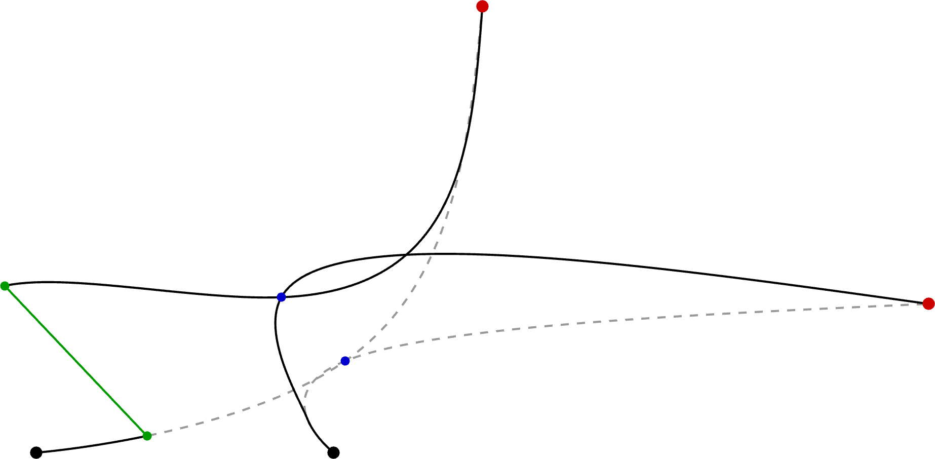
Example with the control of multiple agents
Figure 13 presents an example with the control of multiple agents, with a precision matrix involving nonzero offdiagonal elements. The corresponding example code presents two options: it either requests the two agents to meet in the middle of the motion (e.g., for a handover task), or it requests the two agents to find a location to reach at different time steps (e.g., to drop and pick-up an object), involving nonzero offdiagonal elements at different time steps.
6.6 Dynamical movement primitives (DMP) reformulated as LQT with control primitives
The dynamical movement primitives (DMP) [ 4 ] approach proposes to reproduce an observed movement by crafting a controller composed of two parts: a closed-loop spring-damper system reaching the final point of the observed movement, and an open-loop system reproducing the acceleration profile of the observed movement. These two controllers are weighted so that the spring-damper system part is progressively increased until it becomes the only active controller. In DMP, the acceleration profile (also called forcing terms) is encoded with radial basis functions [ 1 ] , and the spring-damper system parameters are defined heuristically, usually as a critically damped system.
Linear quadratic tracking (LQT) with control primitives can be used in a similar fashion as in DMP, by requesting a target to be reached at the end of the movement and by requesting the observed acceleration profile to be tracked, while encoding the control commands as radial basis functions. The controller can be estimated either as the open-loop control commands ( 55 ), or as the closed-loop controller ( 70 ).
In the latter case, the matrix \bm{F} in ( 71 ) is estimated by using control primitives and an augmented state space formulation, namely
| \bm{\hat{W}}={\big(\bm{\Psi}^{\!{\scriptscriptstyle\top}}\bm{S}_{\bm{u}}^{\scriptscriptstyle\top}\bm{\tilde{Q}}\bm{S}_{\bm{u}}\bm{\Psi}+\bm{\Psi}^{\!{\scriptscriptstyle\top}}\bm{R}\bm{\Psi}\big)}^{-1}\bm{\Psi}^{\!{\scriptscriptstyle\top}}\bm{S}_{\bm{u}}^{\scriptscriptstyle\top}\bm{\tilde{Q}}\bm{S}_{\bm{x}},\quad\bm{F}=\bm{\Psi}\bm{\hat{W}}, |
which is used to compute feedback gains \bm{\tilde{K}}_{t} on the augmented state with ( 72 ).
The resulting controller \bm{\hat{u}}_{t}=-\bm{\tilde{K}}_{t}\bm{\tilde{x}}_{t} tracks the acceleration profile while smoothly reaching the desired goal at the end of the movement, with a smooth transition between the two. The main difference with DMP is that the smooth transition between the two behaviors is directly optimized by the system, and the parameters of the feedback controller are automatically optimized (in DMP, stiffness and damping ratio).
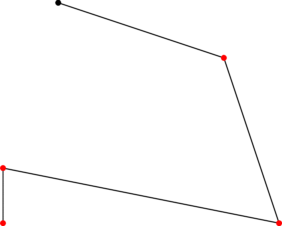
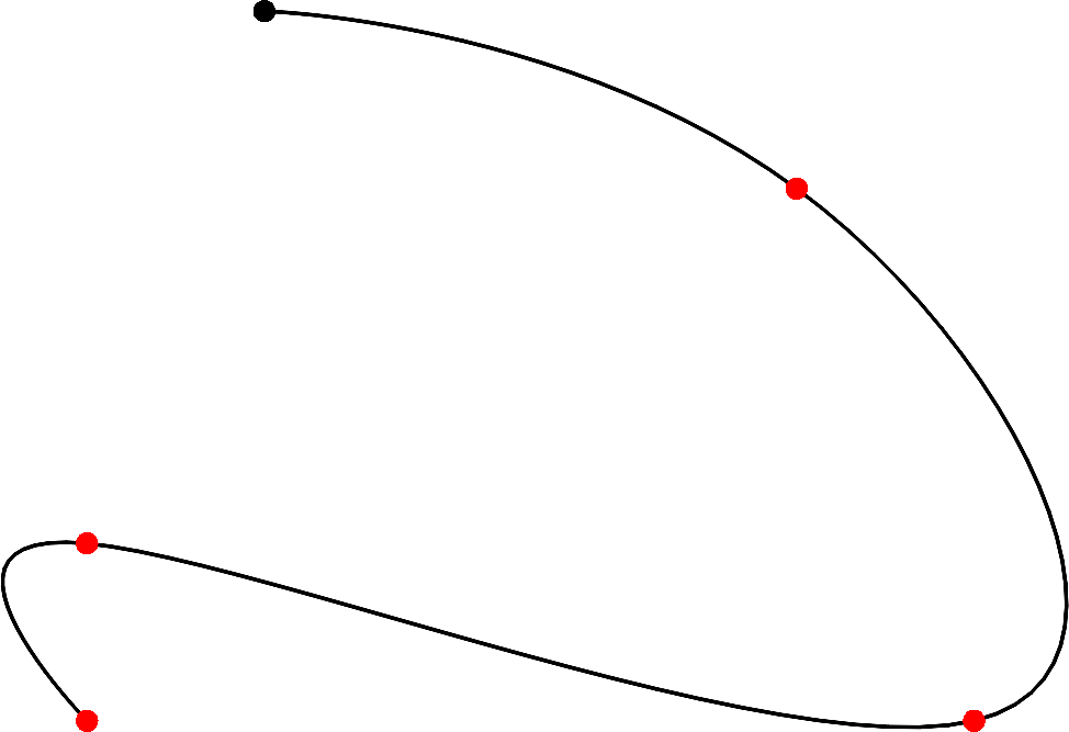
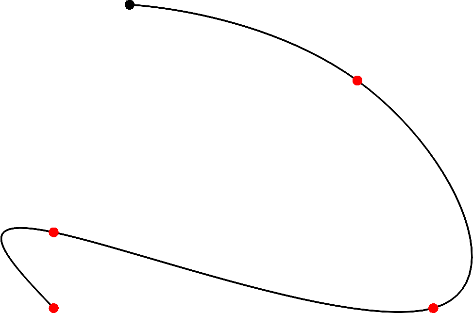
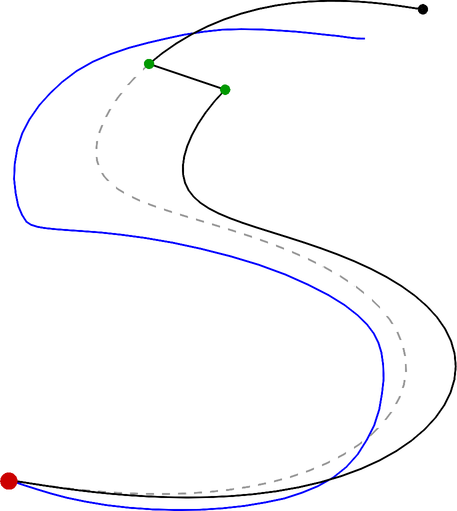
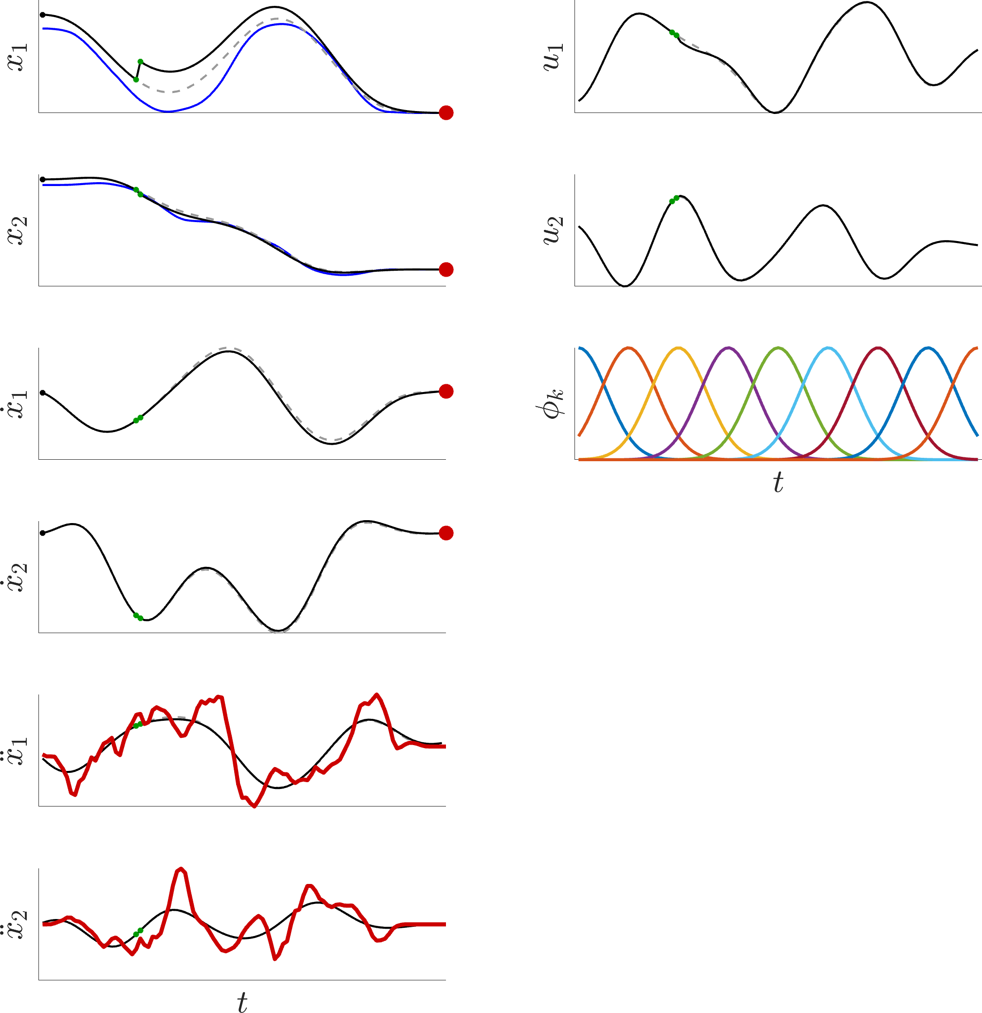
Figure 14 presents an example of reproducing an “S” trajectory with simulation perturbations.
In addition, the LQT formulation allows the resulting controller to be formalized in the form of a cost function, which allows the approach to be combined more fluently with other optimal control strategies. Notably, the approach can be extended to multiple viapoints without any modification. It allows multiple demonstrations of a movement to be used to estimate a feedback controller that will exploit the (co)variations in the demonstrations to provide a minimal intervention control strategy that will selectively reject perturbations based on the impact they can have on the task to achieve. This is effectively attained by automatically regulating the gains in accordance to the variations in the demonstrations, with low gains in parts of the movement allowing variations, and higher gains for parts of the movement that are invariant in the demonstrations. It is also important to highlight that the solution of the LQT problem formulated as in the above is analytical, corresponding to a simple least squares problem.
Moreover, the above problem formulation can be extended to iterative LQR, providing an opportunity to consider obstacle avoidance and constraints within the DMP formulation, as well as to describe costs in task space with a DMP acting in joint angle space.