7 iLQR optimization
Optimal control problems are defined by a cost function \sum_{t=1}^{T}c(\bm{x}_{t},\bm{u}_{t}) to minimize and a dynamical system \bm{x}_{t+1}=\bm{d}(\bm{x}_{t},\bm{u}_{t}) describing the evolution of a state \bm{x}_{t} driven by control commands \bm{u}_{t} during a time window of length T .
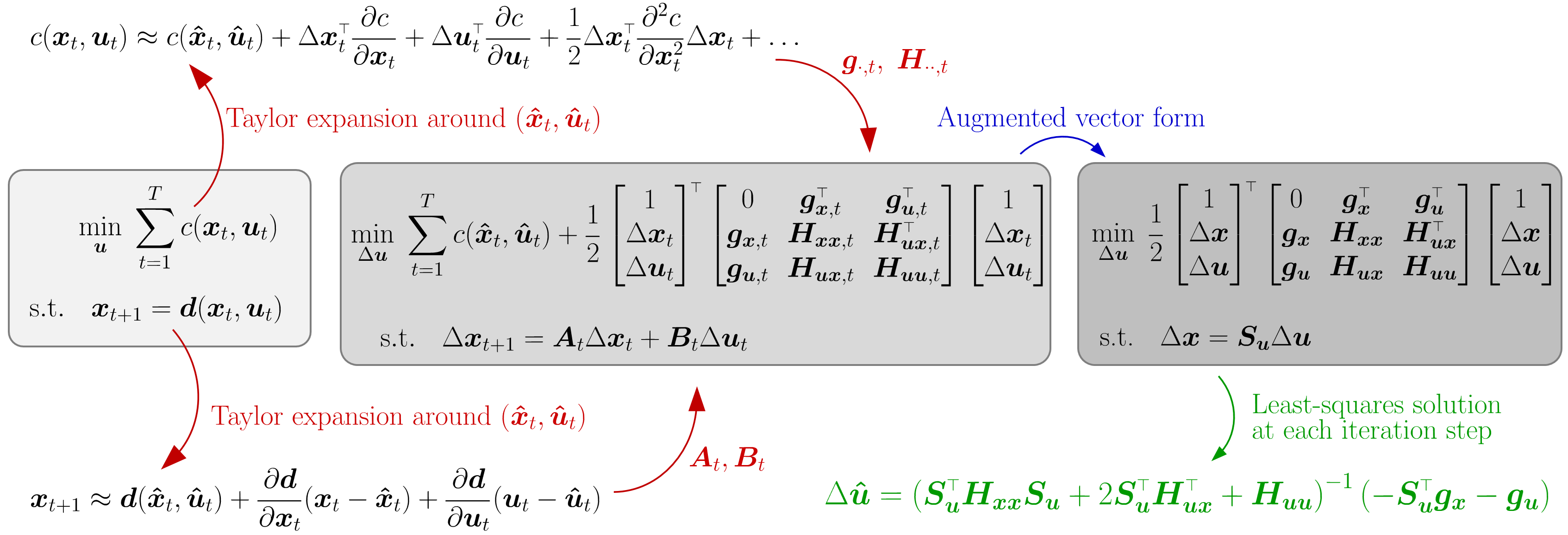
Iterative LQR (iLQR) [ 6 ] solves such constrained nonlinear models by carrying out Taylor expansions on the cost and on the dynamical system so that a solution can be found iteratively by solving a LQR problem at each iteration, similarly to differential dynamic programming approaches [ 8 , 14 ] .
iLQR employs a first order Taylor expansion of the dynamical system \bm{x}_{t+1}=\bm{d}(\bm{x}_{t},\bm{u}_{t}) around the point (\bm{\hat{x}}_{t},\bm{\hat{u}}_{t}) , namely
| \displaystyle\bm{x}_{t+1} | \displaystyle\approx\bm{d}(\bm{\hat{x}}_{t},\bm{\hat{u}}_{t})+\frac{\partial\bm{d}}{\partial\bm{x}_{t}}(\bm{x}_{t}-\bm{\hat{x}}_{t})+\frac{\partial\bm{d}}{\partial\bm{u}_{t}}(\bm{u}_{t}-\bm{\hat{u}}_{t}) | ||
| \displaystyle\iff\Delta\bm{x}_{t+1} | \displaystyle\approx\bm{A}_{t}\Delta\bm{x}_{t}+\bm{B}_{t}\Delta\bm{u}_{t}, |
with residual vectors
| \Delta\bm{x}_{t}\!=\!\bm{x}_{t}\!-\!\bm{\hat{x}}_{t},\quad\Delta\bm{u}_{t}\!=\!\bm{u}_{t}\!-\!\bm{\hat{u}}_{t}, |
and Jacobian matrices
| \bm{A}_{t}=\frac{\partial\bm{d}}{\partial\bm{x}_{t}}\Big|_{\bm{\hat{x}}_{t},\bm{\hat{u}}_{t}},\quad\bm{B}_{t}=\frac{\partial\bm{d}}{\partial\bm{u}_{t}}\Big|_{\bm{\hat{x}}_{t},\bm{\hat{u}}_{t}}. |
The cost function c(\bm{x}_{t},\bm{u}_{t}) for time step t can similarly be approximated by a second order Taylor expansion around the point (\bm{\hat{x}}_{t},\bm{\hat{u}}_{t}) , namely
| \displaystyle c(\bm{x}_{t},\bm{u}_{t}) | \displaystyle\approx c(\bm{\hat{x}}_{t},\bm{\hat{u}}_{t})+\Delta\bm{x}_{t}^{\scriptscriptstyle\top}\frac{\partial c}{\partial\bm{x}_{t}}+\Delta\bm{u}_{t}^{\scriptscriptstyle\top}\frac{\partial c}{\partial\bm{u}_{t}}+\frac{1}{2}\Delta\bm{x}_{t}^{\scriptscriptstyle\top}\frac{\partial^{2}c}{\partial\bm{x}_{t}^{2}}\Delta\bm{x}_{t}+\Delta\bm{x}_{t}^{\scriptscriptstyle\top}\frac{\partial^{2}c}{\partial\bm{x}_{t}\bm{u}_{t}}\Delta\bm{u}_{t}+\frac{1}{2}\Delta\bm{u}_{t}^{\scriptscriptstyle\top}\frac{\partial^{2}c}{\partial\bm{u}_{t}^{2}}\Delta\bm{u}_{t}, | ||
| \displaystyle\iff c(\bm{x}_{t},\bm{u}_{t}) | \displaystyle\approx c(\bm{\hat{x}}_{t},\bm{\hat{u}}_{t})+\frac{1}{2}\begin{bmatrix}1\\ \Delta\bm{x}_{t}\\ \Delta\bm{u}_{t}\end{bmatrix}^{\!{\scriptscriptstyle\top}}\begin{bmatrix}0&\bm{g}_{\bm{x},t}^{\scriptscriptstyle\top}&\bm{g}_{\bm{u},t}^{\scriptscriptstyle\top}\\ \bm{g}_{\bm{x},t}&\bm{H}_{\bm{x}\bm{x},t}&\bm{H}_{\bm{u}\bm{x},t}^{\scriptscriptstyle\top}\\ \bm{g}_{\bm{u},t}&\bm{H}_{\bm{u}\bm{x},t}&\bm{H}_{\bm{u}\bm{u},t}\\ \end{bmatrix}\begin{bmatrix}1\\ \Delta\bm{x}_{t}\\ \Delta\bm{u}_{t}\end{bmatrix}, |
with gradients
| \bm{g}_{\bm{x},t}=\frac{\partial c}{\partial\bm{x}_{t}}\Big|_{\bm{\hat{x}}_{t},\bm{\hat{u}}_{t}},\quad\bm{g}_{\bm{u},t}=\frac{\partial c}{\partial\bm{u}_{t}}\Big|_{\bm{\hat{x}}_{t},\bm{\hat{u}}_{t}}, |
and Hessian matrices
| \bm{H}_{\bm{x}\bm{x},t}=\frac{\partial^{2}c}{\partial\bm{x}_{t}^{2}}\Big|_{\bm{\hat{x}}_{t},\bm{\hat{u}}_{t}},\quad\bm{H}_{\bm{u}\bm{u},t}=\frac{\partial^{2}c}{\partial\bm{u}_{t}^{2}}\Big|_{\bm{\hat{x}}_{t},\bm{\hat{u}}_{t}},\quad\bm{H}_{\bm{u}\bm{x},t}=\frac{\partial^{2}c}{\partial\bm{u}_{t}\partial\bm{x}_{t}}\Big|_{\bm{\hat{x}}_{t},\bm{\hat{u}}_{t}}. |
7.1 Batch formulation of iLQR
A solution in batch form can be computed by minimizing over \bm{u}\!=\!{\begin{bmatrix}\bm{u}_{1}^{\scriptscriptstyle\top},\bm{u}_{2}^{\scriptscriptstyle\top},\ldots,\bm{u}_{T-1}^{\scriptscriptstyle\top}\end{bmatrix}}^{\scriptscriptstyle\top} , yielding a series of open loop control commands \bm{u}_{t} , corresponding to a Gauss–Newton iteration scheme, see Section 2.1 .
At a trajectory level, we denote \bm{x}\!=\!{\begin{bmatrix}\bm{x}_{1}^{\scriptscriptstyle\top},\bm{x}_{2}^{\scriptscriptstyle\top},\ldots,\bm{x}_{T}^{\scriptscriptstyle\top}\end{bmatrix}}^{\scriptscriptstyle\top} the evolution of the state and \bm{u}\!=\!{\begin{bmatrix}\bm{u}_{1}^{\scriptscriptstyle\top},\bm{u}_{2}^{\scriptscriptstyle\top},\ldots,\bm{u}_{T-1}^{\scriptscriptstyle\top}\end{bmatrix}}^{\scriptscriptstyle\top} the evolution of the control commands. The evolution of the state in ( 73 ) becomes \Delta\bm{x}=\bm{S}_{\bm{u}}\Delta\bm{u} , see Appendix A for details. 1 1 1 Note that \bm{S}_{\bm{x}}\Delta\bm{x}_{1}\!=\!\bm{0} because \Delta\bm{x}_{1}\!=\!\bm{0} (as we want our motion to start from \bm{x}_{1} ).
The minimization problem can then be rewritten in batch form as
| \min_{\Delta\bm{u}}\Delta c(\Delta\bm{x},\Delta\bm{u}),\quad\text{s.t.}\quad\Delta\bm{x}=\bm{S}_{\bm{u}}\Delta\bm{u},\quad\text{where}\quad\Delta c(\Delta\bm{x},\Delta\bm{u})=\frac{1}{2}\begin{bmatrix}1\\ \Delta\bm{x}\\ \Delta\bm{u}\end{bmatrix}^{\!{\scriptscriptstyle\top}}\begin{bmatrix}0&\bm{g}_{\bm{x}}^{\scriptscriptstyle\top}&\bm{g}_{\bm{u}}^{\scriptscriptstyle\top}\\ \bm{g}_{\bm{x}}&\bm{H}_{\bm{x}\bm{x}}&\bm{H}_{\bm{u}\bm{x}}^{\scriptscriptstyle\top}\\ \bm{g}_{\bm{u}}&\bm{H}_{\bm{u}\bm{x}}&\bm{H}_{\bm{u}\bm{u}}\\ \end{bmatrix}\begin{bmatrix}1\\ \Delta\bm{x}\\ \Delta\bm{u}\end{bmatrix}. |
By inserting the constraint into the cost, we obtain the optimization problem
| \min_{\Delta\bm{u}}\quad\Delta\bm{u}^{\scriptscriptstyle\top}\bm{S}_{\bm{u}}^{\scriptscriptstyle\top}\bm{g}_{\bm{x}}+\Delta\bm{u}^{\scriptscriptstyle\top}\bm{g}_{\bm{u}}+\frac{1}{2}\Delta\bm{u}^{\scriptscriptstyle\top}\bm{S}_{\bm{u}}^{\scriptscriptstyle\top}\bm{H}_{\bm{x}\bm{x}}\bm{S}_{\bm{u}}\Delta\bm{u}+\Delta\bm{u}^{\scriptscriptstyle\top}\bm{S}_{\bm{u}}^{\scriptscriptstyle\top}\bm{H}_{\bm{u}\bm{x}}^{\scriptscriptstyle\top}\Delta\bm{u}+\frac{1}{2}\Delta\bm{u}^{\scriptscriptstyle\top}\bm{H}_{\bm{u}\bm{u}}\Delta\bm{u}, |
which can be solved analytically by differentiating with respect to \Delta\bm{u} and equating to zero, namely,
| \bm{S}_{\bm{u}}^{\scriptscriptstyle\top}\bm{g}_{\bm{x}}+\bm{g}_{\bm{u}}+\\ \bm{S}_{\bm{u}}^{\scriptscriptstyle\top}\bm{H}_{\bm{x}\bm{x}}\bm{S}_{\bm{u}}\Delta\bm{u}+2\bm{S}_{\bm{u}}^{\scriptscriptstyle\top}\bm{H}_{\bm{u}\bm{x}}^{\scriptscriptstyle\top}\Delta\bm{u}+\bm{H}_{\bm{u}\bm{u}}\Delta\bm{u}=0, |
providing the least squares solution
| \Delta\bm{\hat{u}}={\left(\bm{S}_{\bm{u}}^{\scriptscriptstyle\top}\bm{H}_{\bm{x}\bm{x}}\bm{S}_{\bm{u}}+2\bm{S}_{\bm{u}}^{\scriptscriptstyle\top}\bm{H}_{\bm{u}\bm{x}}^{\scriptscriptstyle\top}+\bm{H}_{\bm{u}\bm{u}}\right)}^{-1}\left(-\bm{S}_{\bm{u}}^{\scriptscriptstyle\top}\bm{g}_{\bm{x}}-\bm{g}_{\bm{u}}\right), |
which can be used to update the control commands estimate at each iteration step of the iLQR algorithm.
The complete iLQR procedure is described in Algorithm 4 (including backtracking line search). Figure 15 also presents an illustrative summary of the iLQR optimization procedure in batch form.
7.2 Recursive formulation of iLQR
A solution can alternatively be computed in a recursive form to provide a controller with feedback gains. Section 6.3 presented the dynamic programming principle in the context of linear quadratic regulation problems, which allowed us to reduce the minimization over an entire sequence of control commands to a sequence of minimization problems over control commands at a single time step, by proceeding backwards in time. In this section, the approach is extended to iLQR.
Similarly to ( 62 ), we have here
| \displaystyle\hat{v}_{t}(\Delta\bm{x}_{t}) | \displaystyle=\min_{\Delta\bm{u}_{t}}\,\underbrace{c_{t}(\Delta\bm{x}_{t},\Delta\bm{u}_{t})+\hat{v}_{t+1}(\Delta\bm{x}_{t+1})}_{q_{t}(\Delta\bm{x}_{t},\Delta\bm{u}_{t})}, |
Similarly to LQR, by starting from the last time step T , \hat{v}_{T}(\Delta\bm{x}_{T}) is independent of the control commands. By relabeling \bm{g}_{\bm{x},T} and \bm{H}_{\bm{x}\bm{x},T} as \bm{v}_{\bm{x},T} and \bm{V}_{\bm{x}\bm{x},T} , we can show that \hat{v}_{T-1} has the same quadratic form as \hat{v}_{T} , enabling the backward recursive computation of \hat{v}_{t} from t=T-1 to t=1 .
This dynamic programming recursion takes the form
| \hat{v}_{t+1}=\begin{bmatrix}1\\ \Delta\bm{x}_{t+1}\end{bmatrix}^{\!{\scriptscriptstyle\top}}\begin{bmatrix}0&\bm{v}_{\bm{x},{t+1}}^{\scriptscriptstyle\top}\\ \bm{v}_{\bm{x},{t+1}}&\bm{V}_{\bm{x}\bm{x},{t+1}}\end{bmatrix}\begin{bmatrix}1\\ \Delta\bm{x}_{t+1}\end{bmatrix}, |
and we then have with ( 79 ) that
| \hat{v}_{t}=\min_{\Delta\bm{u}_{t}}\begin{bmatrix}1\\ \Delta\bm{x}_{t}\\ \Delta\bm{u}_{t}\end{bmatrix}^{\!{\scriptscriptstyle\top}}\begin{bmatrix}0&\bm{g}_{\bm{x},{t}}^{\scriptscriptstyle\top}&\bm{g}_{\bm{u},{t}}^{\scriptscriptstyle\top}\\ \bm{g}_{\bm{x},{t}}&\bm{H}_{\bm{x}\bm{x},{t}}&\bm{H}_{\bm{u}\bm{x},{t}}^{\scriptscriptstyle\top}\\ \bm{g}_{\bm{u},{t}}&\bm{H}_{\bm{u}\bm{x},{t}}&\bm{H}_{\bm{u}\bm{u},{t}}\\ \end{bmatrix}\begin{bmatrix}1\\ \Delta\bm{x}_{t}\\ \Delta\bm{u}_{t}\end{bmatrix}+\begin{bmatrix}1\\ \Delta\bm{x}_{t+1}\end{bmatrix}^{\!{\scriptscriptstyle\top}}\begin{bmatrix}0&\bm{v}_{\bm{x},{t+1}}^{\scriptscriptstyle\top}\\ \bm{v}_{\bm{x},{t+1}}&\bm{V}_{\bm{x}\bm{x},{t+1}}\end{bmatrix}\begin{bmatrix}1\\ \Delta\bm{x}_{t+1}\end{bmatrix}. |
By substituting \Delta\bm{x}_{t+1}=\bm{A}_{t}\Delta\bm{x}_{t}+\bm{B}_{t}\Delta\bm{u}_{t} into ( 81 ), \hat{v}_{t} can be rewritten as
| \hat{v}_{t}=\min_{\Delta\bm{u}_{t}}\begin{bmatrix}1\\ \Delta\bm{x}_{t}\\ \Delta\bm{u}_{t}\end{bmatrix}^{\!\!{\scriptscriptstyle\top}}\!\!\begin{bmatrix}0&\bm{q}_{\bm{x},t}^{\scriptscriptstyle\top}&\bm{q}_{\bm{u},t}^{\scriptscriptstyle\top}\\ \bm{q}_{\bm{x},t}&\bm{Q}_{\bm{x}\bm{x},t}&\bm{Q}_{\bm{u}\bm{x},t}^{\scriptscriptstyle\top}\\ \bm{q}_{\bm{u},t}&\bm{Q}_{\bm{u}\bm{x},t}&\bm{Q}_{\bm{u}\bm{u},t}\\ \end{bmatrix}\!\!\begin{bmatrix}1\\ \Delta\bm{x}_{t}\\ \Delta\bm{u}_{t}\end{bmatrix},\quad\text{where}\quad\left\{\begin{aligned} \bm{q}_{\bm{x},t}&=\bm{g}_{\bm{x},t}+\bm{A}_{t}^{\scriptscriptstyle\top}\bm{v}_{\bm{x},t+1},\\ \bm{q}_{\bm{u},t}&=\bm{g}_{\bm{u},t}+\bm{B}_{t}^{\scriptscriptstyle\top}\,\bm{v}_{\bm{x},t+1},\\ \bm{Q}_{\bm{x}\bm{x},t}&\approx\bm{H}_{\bm{x}\bm{x},t}+\bm{A}_{t}^{\scriptscriptstyle\top}\,\bm{V}_{\bm{x}\bm{x},t+1}\,\bm{A}_{t},\\ \bm{Q}_{\bm{u}\bm{u},t}&\approx\bm{H}_{\bm{u}\bm{u},t}+\bm{B}_{t}^{\scriptscriptstyle\top}\,\bm{V}_{\bm{x}\bm{x},t+1}\,\bm{B}_{t},\\ \bm{Q}_{\bm{u}\bm{x},t}&\approx\bm{H}_{\bm{u}\bm{x},t}+\bm{B}_{t}^{\scriptscriptstyle\top}\,\bm{V}_{\bm{x}\bm{x},t+1}\,\bm{A}_{t},\end{aligned}\right. |
with gradients
| \bm{g}_{\bm{x},t}=\frac{\partial c}{\partial\bm{x}_{t}}\Big|_{\bm{\hat{x}}_{t},\bm{\hat{u}}_{t}},\quad\bm{g}_{\bm{u},t}=\frac{\partial c}{\partial\bm{u}_{t}}\Big|_{\bm{\hat{x}}_{t},\bm{\hat{u}}_{t}},\quad\bm{v}_{\bm{x},t}=\frac{\partial\hat{v}}{\partial\bm{x}_{t}}\Big|_{\bm{\hat{x}}_{t},\bm{\hat{u}}_{t}},\quad\bm{q}_{\bm{x},t}=\frac{\partial q}{\partial\bm{x}_{t}}\Big|_{\bm{\hat{x}}_{t},\bm{\hat{u}}_{t}},\quad\bm{q}_{\bm{u},t}=\frac{\partial q}{\partial\bm{u}_{t}}\Big|_{\bm{\hat{x}}_{t},\bm{\hat{u}}_{t}}, |
Jacobian matrices
| \bm{A}_{t}=\frac{\partial\bm{d}}{\partial\bm{x}_{t}}\Big|_{\bm{\hat{x}}_{t},\bm{\hat{u}}_{t}},\quad\bm{B}_{t}=\frac{\partial\bm{d}}{\partial\bm{u}_{t}}\Big|_{\bm{\hat{x}}_{t},\bm{\hat{u}}_{t}}, |
and Hessian matrices
| \bm{H}_{\bm{x}\bm{x},t}\!=\!\frac{\partial^{2}c}{\partial\bm{x}_{t}^{2}}\Big|_{\bm{\hat{x}}_{t},\bm{\hat{u}}_{t}},\quad\bm{H}_{\bm{u}\bm{u},t}\!=\!\frac{\partial^{2}c}{\partial\bm{u}_{t}^{2}}\Big|_{\bm{\hat{x}}_{t},\bm{\hat{u}}_{t}},\quad\bm{H}_{\bm{u}\bm{x},t}\!=\!\frac{\partial^{2}c}{\partial\bm{u}_{t}\partial\bm{x}_{t}}\Big|_{\bm{\hat{x}}_{t},\bm{\hat{u}}_{t}},\quad\bm{V}_{\bm{x}\bm{x},t}\!=\!\frac{\partial^{2}\hat{v}}{\partial\bm{x}_{t}^{2}}\Big|_{\bm{\hat{x}}_{t},\bm{\hat{u}}_{t}}, |
| \bm{Q}_{\bm{x}\bm{x},t}=\frac{\partial^{2}q}{\partial\bm{x}_{t}^{2}}\Big|_{\bm{\hat{x}}_{t},\bm{\hat{u}}_{t}},\quad\bm{Q}_{\bm{u}\bm{u},t}=\frac{\partial^{2}q}{\partial\bm{u}_{t}^{2}}\Big|_{\bm{\hat{x}}_{t},\bm{\hat{u}}_{t}},\quad\bm{Q}_{\bm{u}\bm{x},t}=\frac{\partial^{2}q}{\partial\bm{u}_{t}\partial\bm{x}_{t}}\Big|_{\bm{\hat{x}}_{t},\bm{\hat{u}}_{t}}. |
Minimizing ( 82 ) w.r.t. \Delta\bm{u}_{t} can be achieved by differentiating the equation and equating to zero, yielding the controller
| \Delta\bm{\hat{u}}_{t}=\bm{k}_{t}+\bm{K}_{t}\,\Delta\bm{x}_{t},\;\text{with}\quad\left\{\begin{aligned} \bm{k}_{t}&=-\bm{Q}_{\bm{u}\bm{u},t}^{-1}\,\bm{q}_{\bm{u},t},\\ \bm{K}_{t}&=-\bm{Q}_{\bm{u}\bm{u},t}^{-1}\,\bm{Q}_{\bm{u}\bm{x},t},\end{aligned}\right. |
where \bm{k}_{t} is a feedforward command and \bm{K}_{t} is a feedback gain matrix.
By inserting ( 83 ) into ( 82 ), we get the recursive updates
| \displaystyle\bm{v}_{\bm{x},t} | \displaystyle=\bm{q}_{\bm{x},t}-\bm{Q}_{\bm{u}\bm{x},t}^{\scriptscriptstyle\top}\,\bm{Q}_{\bm{u}\bm{u},t}^{-1}\,\bm{q}_{\bm{u},t}, | ||
| \displaystyle\bm{V}_{\bm{x}\bm{x},t} | \displaystyle=\bm{Q}_{\bm{x}\bm{x},t}-\bm{Q}_{\bm{u}\bm{x},t}^{\scriptscriptstyle\top}\,\bm{Q}_{\bm{u}\bm{u},t}^{-1}\,\bm{Q}_{\bm{u}\bm{x},t}. |
In this recursive iLQR formulation, at each iteration step of the optimization algorithm, the nominal trajectories (\bm{\hat{x}}_{t},\bm{\hat{u}}_{t}) are refined, together with feedback matrices \bm{K}_{t} . Thus, at each iteration step of the optimization algorithm, a backward and forward recursion is performed to evaluate these vectors and matrices. There is thus two types of iterations: one for the optimization algorithm, and one for the dynamic programming recursion performed at each given iteration.
After convergence, by using ( 83 ) and the nominal trajectories in the state and control spaces (\bm{\hat{x}}_{t},\bm{\hat{u}}_{t}) , the resulting controller at each time step t is
| \bm{u}_{t}=\bm{\hat{u}}_{t}+\bm{K}_{t}\,(\bm{\hat{x}}_{t}-\bm{x}_{t}), |
where the evolution of the state is described by \bm{x}_{t+1}=\bm{d}(\bm{x}_{t},\bm{u}_{t}) .
The complete iLQR procedure is described in Algorithm 5 (including backtracking line search).
7.3 Least squares formulation of recursive iLQR
First, note that ( 83 ) can be rewritten as
| \Delta\bm{\hat{u}}_{t}=\bm{\tilde{K}}_{t}\,\begin{bmatrix}\Delta\bm{x}_{t}\\ 1\end{bmatrix},\;\text{with}\quad\bm{\tilde{K}}_{t}=-\bm{Q}_{\bm{u}\bm{u},t}^{-1}\Big[\bm{Q}_{\bm{u}\bm{x},t},\;\bm{q}_{\bm{u},t}\Big]. |
Also, ( 76 ) can be rewritten as
| \min_{\Delta\bm{u}}\quad\underbrace{\frac{1}{2}\begin{bmatrix}\Delta\bm{u}\\ 1\end{bmatrix}^{\scriptscriptstyle\top}\begin{bmatrix}\bm{C}&\bm{c}\\ \bm{c}^{\scriptscriptstyle\top}&0\end{bmatrix}\begin{bmatrix}\Delta\bm{u}\\ 1\end{bmatrix}}_{\frac{1}{2}\Delta\bm{u}^{\scriptscriptstyle\top}\bm{C}\Delta\bm{u}+\Delta\bm{u}^{\scriptscriptstyle\top}\bm{c}},\quad\text{where}\quad\left\{\begin{aligned} \bm{c}&=\bm{S}_{\bm{u}}^{\scriptscriptstyle\top}\bm{g}_{\bm{x}}+\bm{g}_{\bm{u}},\\ \bm{C}&=\bm{S}_{\bm{u}}^{\scriptscriptstyle\top}\bm{H}_{\bm{x}\bm{x}}\bm{S}_{\bm{u}}+2\bm{S}_{\bm{u}}^{\scriptscriptstyle\top}\bm{H}_{\bm{u}\bm{x}}^{\scriptscriptstyle\top}+\bm{H}_{\bm{u}\bm{u}}.\end{aligned}\right. |
Similarly to Section 6.5 , we set
| \Delta\bm{u}=-\bm{F}\begin{bmatrix}\Delta\bm{x}_{1}\\ 1\end{bmatrix}=-\bm{F}\begin{bmatrix}\bm{0}\\ 1\end{bmatrix}=-\bm{F}\Delta\bm{\tilde{x}}_{1}, |
and redefine the optimization problem as
| \min_{\bm{F}}\quad\frac{1}{2}\Delta\bm{\tilde{x}}_{1}^{\scriptscriptstyle\top}\bm{F}^{\scriptscriptstyle\top}\bm{C}\bm{F}\Delta\bm{\tilde{x}}_{1}-\Delta\bm{\tilde{x}}_{1}^{\scriptscriptstyle\top}\bm{F}^{\scriptscriptstyle\top}\bm{c}. |
By differentiating w.r.t. \bm{F} and equating to zero, we get
| \bm{F}\Delta\bm{\tilde{x}}_{1}=\bm{C}^{-1}\bm{c}. |
Similarly to Section 6.5 , we decompose \bm{F} as block matrices \bm{F}_{t} with t\in\{1,\ldots,T-1\} . \bm{F} can then be used to iteratively reconstruct regulation gains \bm{K}_{t} , by starting from \bm{K}_{1}=\bm{F}_{1} , \bm{P}_{1}=\bm{I} , and by computing with forward recursion
| \bm{P}_{t}=\bm{P}_{t-1}{(\bm{A}_{t-1}-\bm{B}_{t-1}\bm{K}_{t-1})}^{-1},\quad\bm{K}_{t}=\bm{F}_{t}\;\bm{P}_{t}, |
from t=2 to t=T-1 .
7.4 Updates by considering step sizes
To be more efficient, iLQR most often requires at each iteration to estimate a step size \alpha to scale the control command updates. For the batch formulation in Section 7.1 , this can be achieved by setting the update ( 78 ) as
| \bm{\hat{u}}\leftarrow\bm{\hat{u}}+\alpha\;\Delta\bm{\hat{u}}, |
where the resulting procedure consists of estimating a descent direction with ( 78 ) along which the objective function will be reduced, and then estimating with ( 91 ) a step size that determines how far one can move along this direction.
For the recursive formulation in Section 7.2 , this can be achieved by setting the update ( 83 ) as
| \bm{\hat{u}}_{t}\leftarrow\bm{\hat{u}}_{t}+\alpha\;\bm{k}_{t}+\bm{K}_{t}\,\Delta\bm{x}_{t}. |
In practice, a simple backtracking line search procedure can be considered with Algorithm 3 , by considering a small value for \alpha_{\min} . For more elaborated methods, see Ch. 3 of [ 10 ] .
The complete iLQR procedures are described in Algorithms 4 and 5 for the batch and recursive formulations, respectively.
7.5 iLQR with quadratic cost on f(x_{t})
We consider a cost defined by
| c(\bm{x}_{t},\bm{u}_{t})=\bm{f}(\bm{x}_{t})^{\!{\scriptscriptstyle\top}}\bm{Q}_{t}\bm{f}(\bm{x}_{t})+\bm{u}_{t}^{\scriptscriptstyle\top}\bm{R}_{t}\,\bm{u}_{t}, |
where \bm{Q}_{t} and \bm{R}_{t} are weight matrices trading off task and control costs. Such cost is quadratic on \bm{f}(\bm{x}_{t}) but non-quadratic on \bm{x}_{t} .
For the batch formulation of iLQR, the cost in ( 74 ) then becomes
| \Delta c(\Delta\bm{x}_{t},\Delta\bm{u}_{t})\approx 2\Delta\bm{x}_{t}^{\scriptscriptstyle\top}\bm{J}(\bm{x}_{t})^{\scriptscriptstyle\top}\bm{Q}_{t}\bm{f}(\bm{x}_{t})+2\Delta\bm{u}_{t}^{\scriptscriptstyle\top}\bm{R}_{t}\,\bm{u}_{t}+\Delta\bm{x}_{t}^{\scriptscriptstyle\top}\bm{J}(\bm{x}_{t})^{\scriptscriptstyle\top}\bm{Q}_{t}\bm{J}(\bm{x}_{t})\Delta\bm{x}_{t}+\Delta\bm{u}_{t}^{\scriptscriptstyle\top}\bm{R}_{t}\Delta\bm{u}_{t}, |
which used gradients
| \bm{g}_{\bm{x},t}=2\bm{J}(\bm{x}_{t})^{\scriptscriptstyle\top}\bm{Q}_{t}\bm{f}(\bm{x}_{t}),\quad\bm{g}_{\bm{u},t}=2\bm{R}_{t}\bm{u}_{t}, |
and Hessian matrices
| \bm{H}_{\bm{x}\bm{x},t}\approx 2\bm{J}(\bm{x}_{t})^{\scriptscriptstyle\top}\bm{Q}_{t}\bm{J}(\bm{x}_{t}),\quad\bm{H}_{\bm{u}\bm{x},t}=\bm{0},\quad\bm{H}_{\bm{u}\bm{u},t}=2\bm{R}_{t}. |
with \bm{J}(\bm{x}_{t})=\frac{\partial\bm{f}(\bm{x}_{t})}{\partial\bm{x}_{t}} a Jacobian matrix. The same results can be used in the recursive formulation in ( 82 ).
At a trajectory level, the evolution of the tracking and control weights is represented by \bm{Q}\!=\!\mathrm{blockdiag}(\bm{Q}_{1},\bm{Q}_{2},\ldots,\bm{Q}_{T}) and \bm{R}\!=\!\mathrm{blockdiag}(\bm{R}_{1},\bm{R}_{2},\ldots,\bm{R}_{T-1}) , respectively.
With a slight abuse of notation, we define \bm{f}(\bm{x}) as a vector concatenating the vectors \bm{f}(\bm{x}_{t}) , and \bm{J}(\bm{x}) as a block-diagonal concatenation of the Jacobian matrices \bm{J}(\bm{x}_{t}) . The minimization problem ( 76 ) then becomes
| \min_{\Delta\bm{u}}\quad 2\Delta\bm{x}^{\!{\scriptscriptstyle\top}}\bm{J}(\bm{x})^{\scriptscriptstyle\top}\bm{Q}\bm{f}(\bm{x})+2\Delta\bm{u}^{\!{\scriptscriptstyle\top}}\bm{R}\,\bm{u}\;+\Delta\bm{x}^{\!{\scriptscriptstyle\top}}\bm{J}(\bm{x})^{\scriptscriptstyle\top}\bm{Q}\bm{J}(\bm{x})\Delta\bm{x}+\Delta\bm{u}^{\!{\scriptscriptstyle\top}}\bm{R}\Delta\bm{u},\quad\text{s.t.}\quad\Delta\bm{x}=\bm{S}_{\bm{u}}\Delta\bm{u}, |
whose least squares solution is given by
| \Delta\bm{\hat{u}}\!=\!{\Big(\bm{S}_{\bm{u}}^{\scriptscriptstyle\top}\bm{J}(\bm{x})^{\scriptscriptstyle\top}\bm{Q}\bm{J}(\bm{x})\bm{S}_{\bm{u}}\!+\!\bm{R}\Big)}^{\!\!-1}\Big(-\bm{S}_{\bm{u}}^{\scriptscriptstyle\top}\bm{J}(\bm{x})^{\scriptscriptstyle\top}\bm{Q}\bm{f}(\bm{x})-\bm{R}\,\bm{u}\Big), |
which can be used to update the control commands estimates at each iteration step of the iLQR algorithm.
In the next sections, we show examples of functions \bm{f}(\bm{x}) that can rely on this formulation.
7.5.1 Robot manipulator
We define a manipulation task involving a set of transformations as in Fig. 16 . By relying on these transformation operators, we will next describe all variables in the robot frame of reference (defined by \bm{0} , \bm{e}_{1} and \bm{e}_{2} in the figure).
For a manipulator controlled by joint angle velocity commands \bm{u}=\bm{\dot{x}} , the evolution of the system is described by \bm{x}_{t+1}=\bm{x}_{t}+\bm{u}_{t}\Delta t , with the Taylor expansion ( 73 ) simplifying to \bm{A}_{t}=\frac{\partial\bm{g}}{\partial\bm{x}_{t}}=\bm{I} and \bm{B}_{t}=\frac{\partial\bm{g}}{\partial\bm{u}_{t}}=\bm{I}\Delta t . Similarly, a double integrator can alternatively be considered, with acceleration commands \bm{u}=\bm{\ddot{x}} and states composed of both positions and velocities.
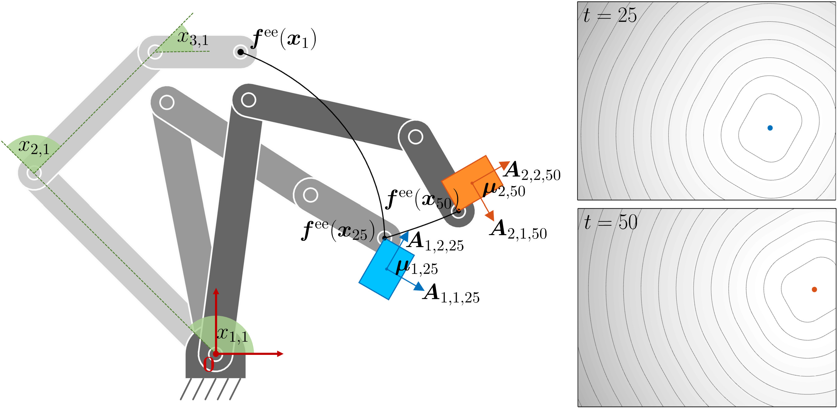
For a robot manipulator, \bm{f}(\bm{x}_{t}) in ( 98 ) typically represents the error between a reference \bm{\mu}_{t} and the end-effector position computed by the forward kinematics function \bm{f}^{\text{\tiny ee}}(\bm{x}_{t}) . We then have
| \displaystyle\bm{f}(\bm{x}_{t}) | \displaystyle=\bm{f}^{\text{\tiny ee}}(\bm{x}_{t})-\bm{\mu}_{t}, | ||
| \displaystyle\bm{J}(\bm{x}_{t}) | \displaystyle=\bm{J}^{\text{\tiny ee}}(\bm{x}_{t}). |
For the orientation part of the data (if considered), the Euclidean distance vector \bm{f}^{\text{\tiny ee}}(\bm{x}_{t})-\bm{\mu}_{t} is replaced by a geodesic distance measure computed with the logarithmic map \log_{\bm{\mu}_{t}}\!\big(\bm{f}^{\text{\tiny ee}}(\bm{x}_{t})\big) , see [ 3 ] for details.
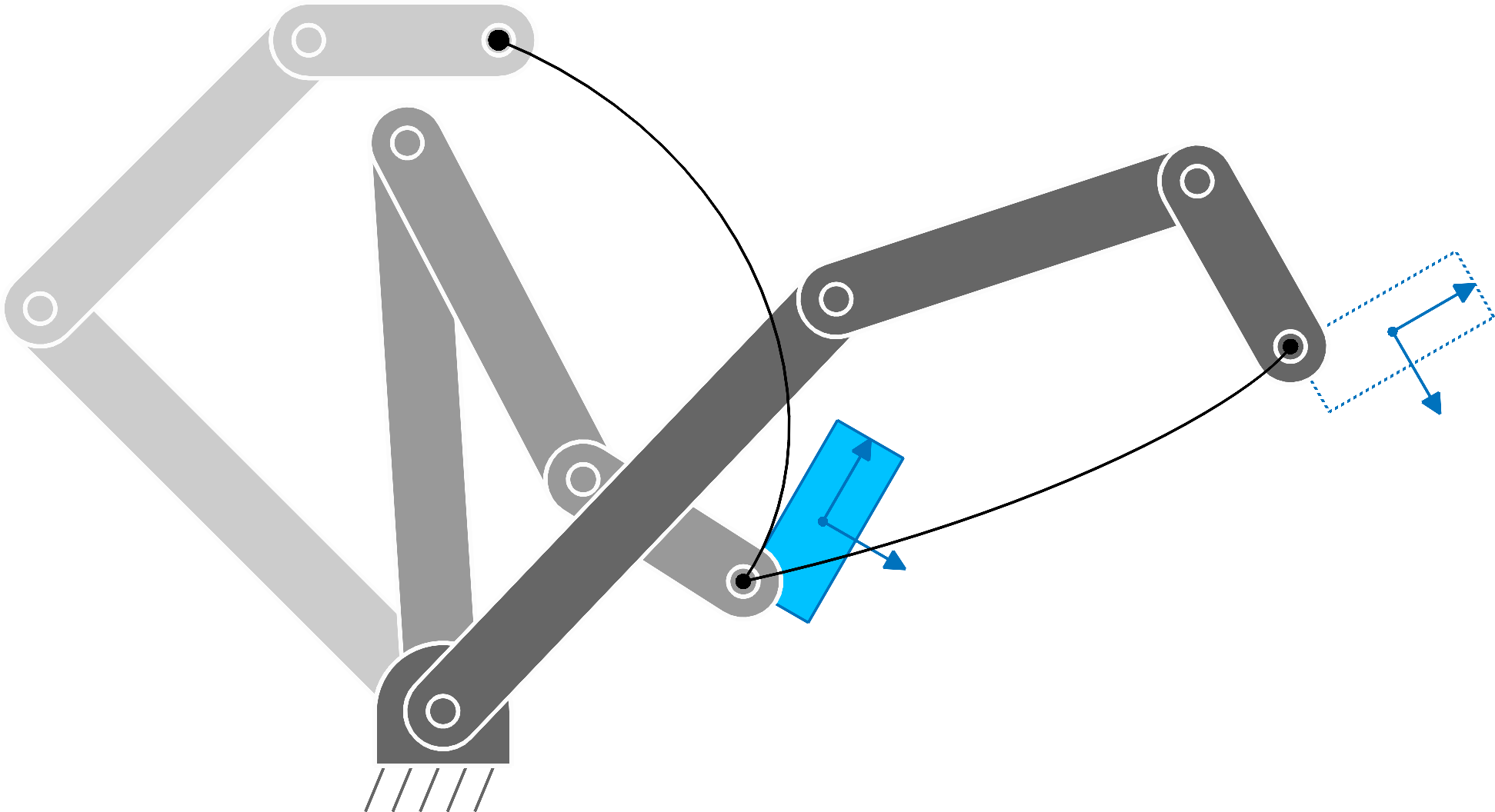
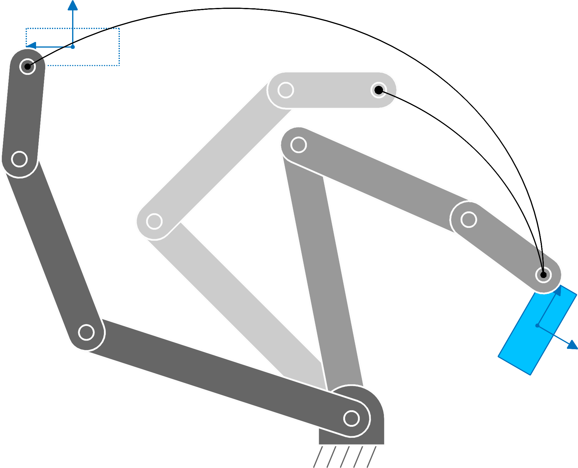
The approach can similarly be extended to target objects/landmarks with positions \bm{\mu}_{t} and orientation matrices \bm{U}_{t} , whose columns are basis vectors forming a coordinate system, see Fig. 18 . We can then define an error between the robot end-effector and an object/landmark expressed in the object/landmark coordinate system as
| \displaystyle\bm{f}(\bm{x}_{t}) | \displaystyle=\bm{U}_{t}^{\scriptscriptstyle\top}\big(\bm{f}^{\text{\tiny ee}}(\bm{x}_{t})-\bm{\mu}_{t}\big), | ||
| \displaystyle\bm{J}(\bm{x}_{t}) | \displaystyle=\bm{U}_{t}^{\scriptscriptstyle\top}\bm{J}^{\text{\tiny ee}}(\bm{x}_{t}). |
7.5.2 Bounded joint space
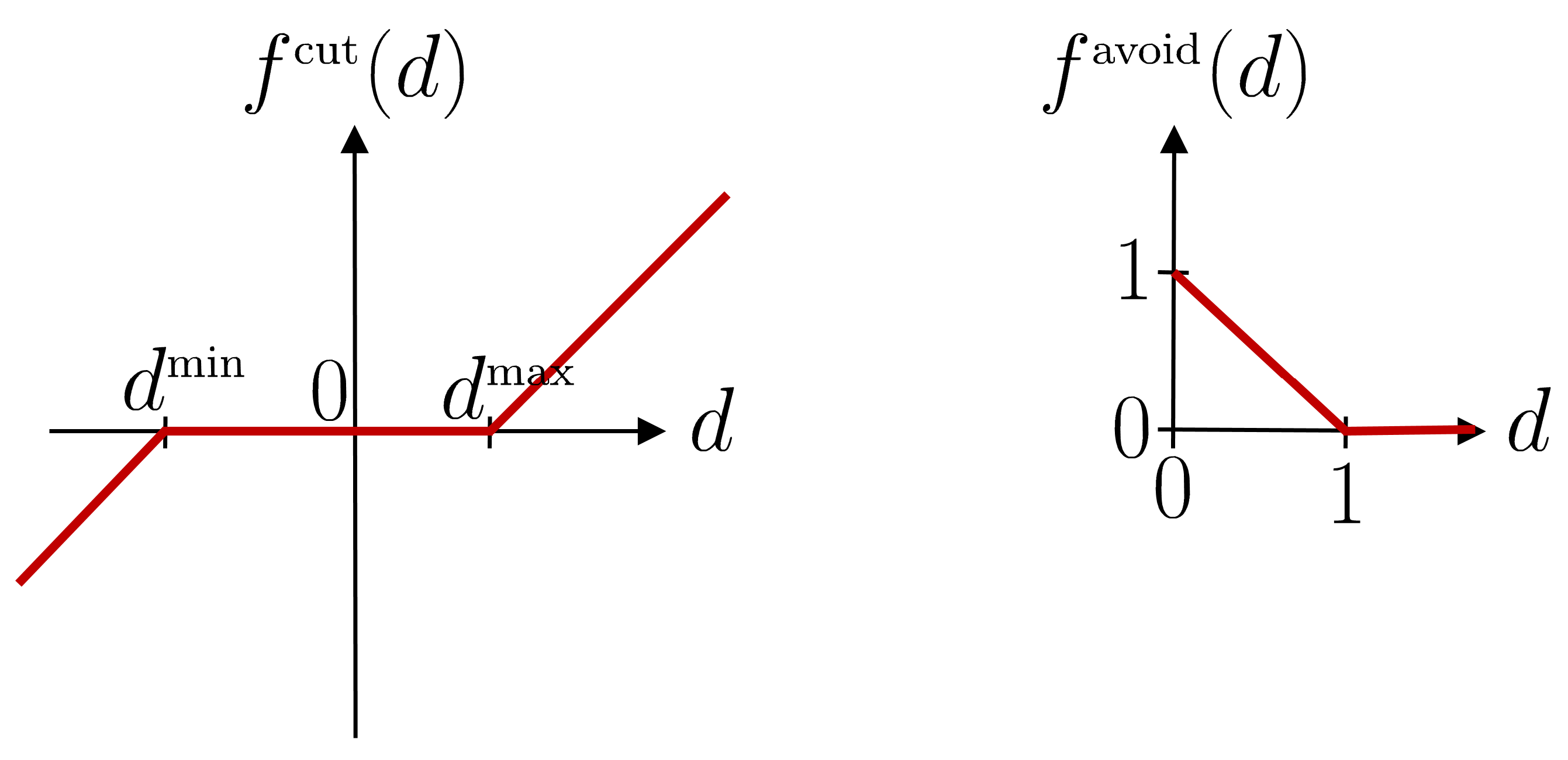
The iLQR solution in ( 98 ) can be used to keep the state within a boundary (e.g., joint angle limits). We denote \bm{f}(\bm{x})=\bm{f}^{\text{\tiny cut}}(\bm{x}) as the vertical concatenation of \bm{f}^{\text{\tiny cut}}(\bm{x}_{t}) and \bm{J}(\bm{x})=\bm{J}^{\text{\tiny cut}}(\bm{x}) as a diagonal concatenation of diagonal Jacobian matrices \bm{J}^{\text{\tiny cut}}(\bm{x}_{t}) . Each element i of \bm{f}^{\text{\tiny cut}}(\bm{x}_{t}) and \bm{J}^{\text{\tiny cut}}(\bm{x}_{t}) is defined as
| \displaystyle f^{\text{\tiny cut}}_{i}(x_{t,i}) | \displaystyle=\begin{cases}\textstyle x_{t,i}-x_{i}^{\scriptscriptstyle\min},&\text{if}\ x_{t,i}<x_{i}^{\scriptscriptstyle\min}\\ \textstyle x_{t,i}-x_{i}^{\scriptscriptstyle\max},&\text{if}\ x_{t,i}>x_{i}^{\scriptscriptstyle\max}\\ \textstyle 0,&\text{otherwise}\end{cases}, | ||
| \displaystyle J^{\text{\tiny cut}}_{i,i}(x_{t,i}) | \displaystyle=\begin{cases}\textstyle 1,\hskip 39.833858pt&\text{if}\ x_{t,i}<x_{i}^{\scriptscriptstyle\min}\\ \textstyle 1,&\text{if}\ x_{t,i}>x_{i}^{\scriptscriptstyle\max}\\ \textstyle 0,&\text{otherwise}\end{cases}, |
where f^{\text{\tiny cut}}_{i}(x_{t,i}) describes continuous ReLU-like functions for each dimension. f^{\text{\tiny cut}}_{i}(x_{t,i}) is 0 inside the bounded domain and takes the signed distance value outside the boundary, see Fig. 17 - left .
We can see with ( 95 ) that for \bm{Q}=\frac{1}{2}\bm{I} , if \bm{x} is outside the domain during some time steps t , \bm{g}_{\bm{x}}=\frac{\partial c}{\partial\bm{x}}=2{\bm{J}}^{\scriptscriptstyle\top}\bm{Q}\bm{f} generates a vector bringing it back to the boundary of the domain.
7.5.3 Bounded task space
The iLQR solution in ( 98 ) can be used to keep the end-effector within a boundary (e.g., end-effector position limits). Based on the above definitions, \bm{f}(\bm{x}) and \bm{J}(\bm{x}) are in this case defined as
| \displaystyle\bm{f}(\bm{x}_{t}) | \displaystyle=\bm{f}^{\text{\tiny cut}}\Big(\bm{e}(\bm{x}_{t})\Big), | ||
| \displaystyle\bm{J}(\bm{x}_{t}) | \displaystyle=\bm{J}^{\text{\tiny cut}}\Big(\bm{e}(\bm{x}_{t})\Big)\;\bm{J}^{\text{\tiny ee}}(\bm{x}_{t}), | ||
| \displaystyle\text{with}\quad\bm{e}(\bm{x}_{t}) | \displaystyle=\bm{f}^{\text{\tiny ee}}(\bm{x}_{t}). |
7.5.4 Reaching task with robot manipulator and prismatic object boundaries
The definition of \bm{f}(\bm{x}_{t}) and \bm{J}(\bm{x}_{t}) in ( 99 ) can also be extended to objects/landmarks with boundaries by defining
| \displaystyle\bm{f}(\bm{x}_{t}) | \displaystyle=\bm{f}^{\text{\tiny cut}}\Big(\bm{e}(\bm{x}_{t})\Big), | ||
| \displaystyle\bm{J}(\bm{x}_{t}) | \displaystyle=\bm{J}^{\text{\tiny cut}}\Big(\bm{e}(\bm{x}_{t})\Big)\;\bm{U}_{t}^{\scriptscriptstyle\top}\;\bm{J}^{\text{\tiny ee}}(\bm{x}_{t}), | ||
| \displaystyle\text{with}\quad\bm{e}(\bm{x}_{t}) | \displaystyle=\bm{U}_{t}^{\scriptscriptstyle\top}\big(\bm{f}^{\text{\tiny ee}}(\bm{x}_{t})-\bm{\mu}_{t}\big), |
see also Fig. 18 .
7.5.5 Center of mass
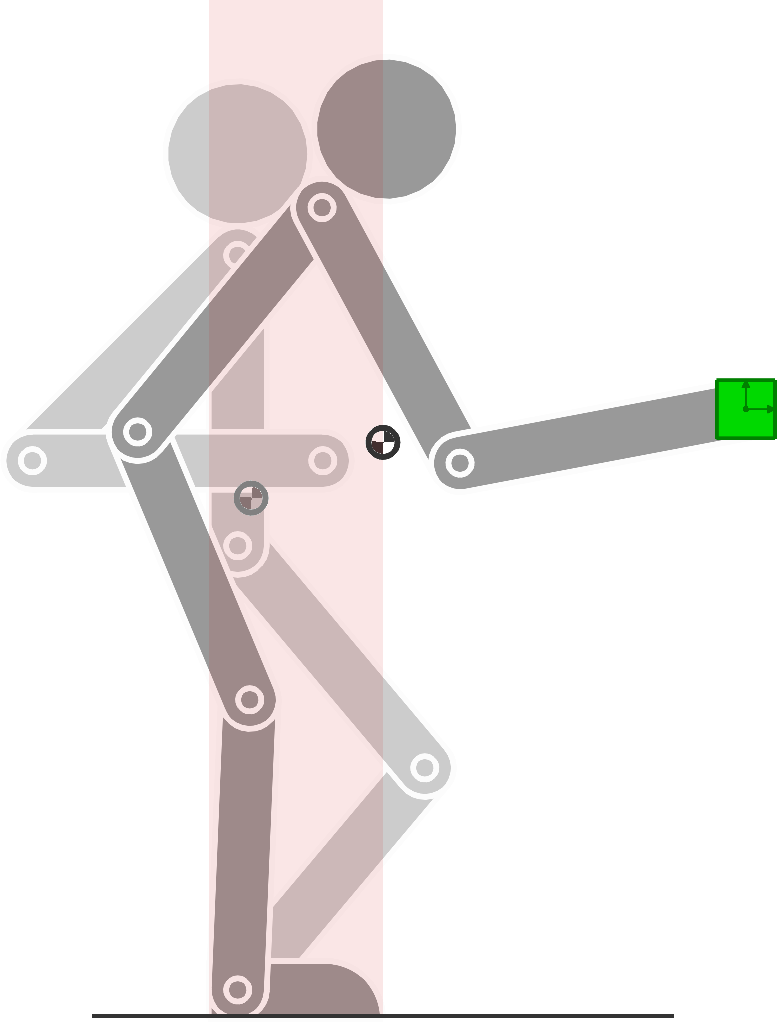
If we assume an equal mass for each link concentrated at the joint (i.e., assuming that the motors and gripper are heavier than the link structures), the forward kinematics function to determine the center of a mass of an articulated chain can simply be computed with
| \bm{f}^{\text{\tiny CoM}}=\frac{1}{D}\begin{bmatrix}\bm{\ell}^{\scriptscriptstyle\top}\bm{L}\cos(\bm{L}\bm{x})\\ \bm{\ell}^{\scriptscriptstyle\top}\bm{L}\sin(\bm{L}\bm{x})\end{bmatrix}, |
which corresponds to the row average of \tilde{f} in ( 13 ) for the first two columns (position). The corresponding Jacobian matrix is
| \bm{J}^{\text{\tiny CoM}}=\frac{1}{D}\begin{bmatrix}-\sin(\bm{L}\bm{x})^{\scriptscriptstyle\top}\bm{L}\;\mathrm{diag}(\bm{\ell}^{\scriptscriptstyle\top}\bm{L})\\ \cos(\bm{L}\bm{x})^{\scriptscriptstyle\top}\bm{L}\;\mathrm{diag}(\bm{\ell}^{\scriptscriptstyle\top}\bm{L})\end{bmatrix}. |
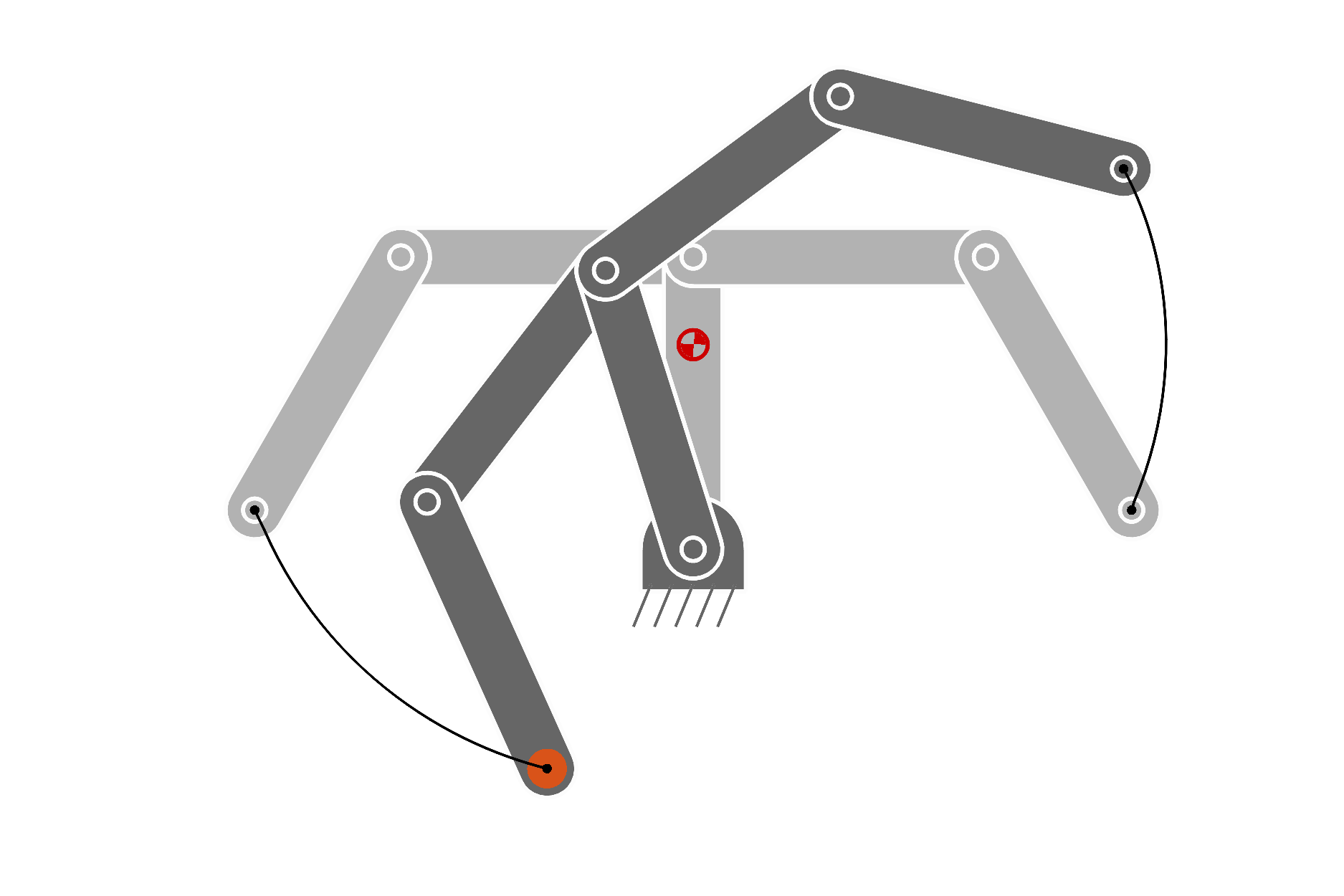
The forward kinematics function \bm{f}^{\text{\tiny CoM}} can be used in tracking tasks similar to the ones considering the end-effector, as in Section 7.5.4 . Fig. 19 shows an example in which the starting and ending poses are depicted in different grayscale levels. The corresponding center of mass is depicted by a darker semi-filled disc. The area allowed for the center of mass is depicted as a transparent red rectangle. The task consists of reaching the green object with the end-effector at the end of the movement, while always keeping the center of mass within the desired bounding box during the movement.
7.5.6 Bimanual robot
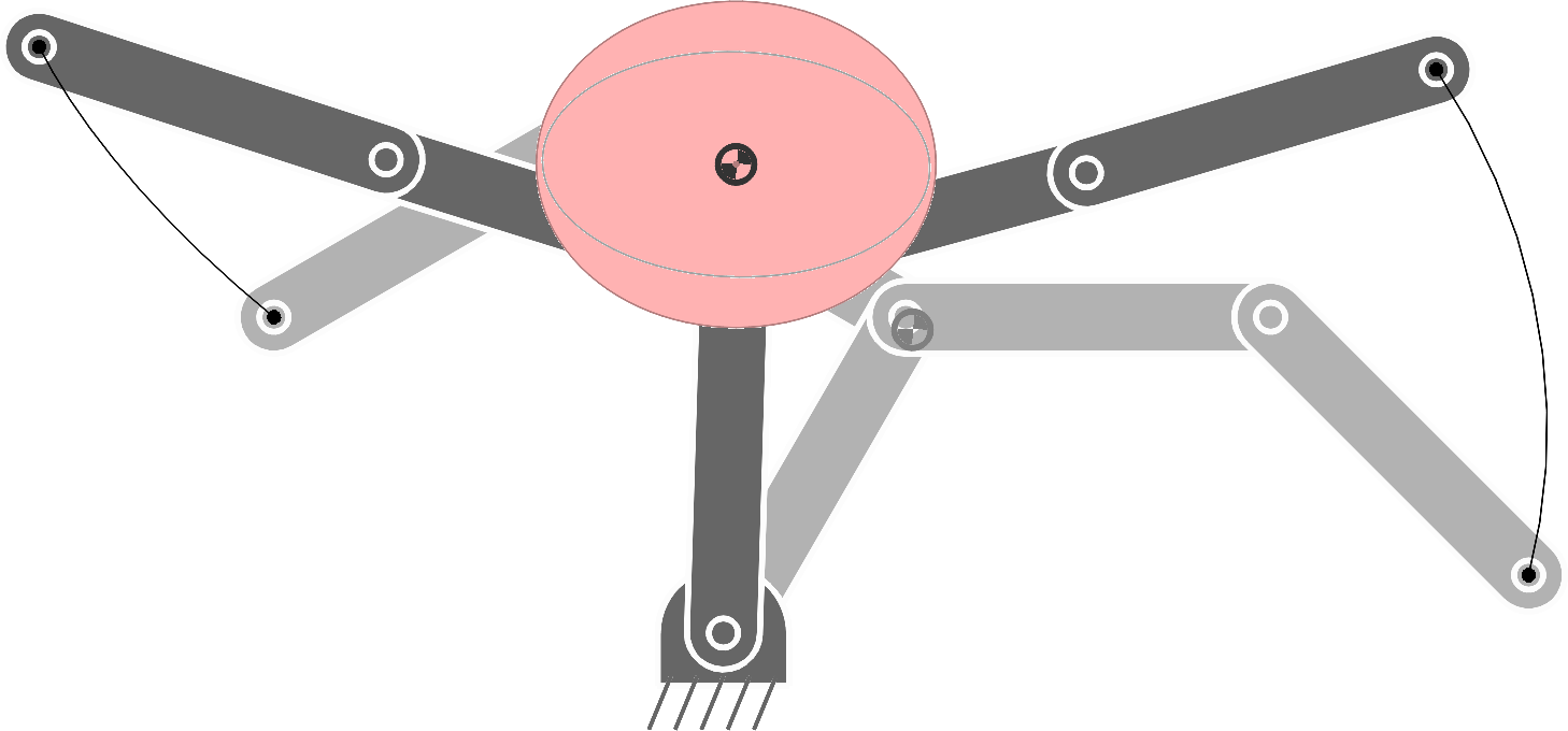
We consider a 5-link planar bimanual robot with a torso link shared by the two arms, see Fig. 20 . We define the forward kinematics function as
| \bm{f}=\begin{bmatrix}\bm{\ell}_{\scriptscriptstyle{[1,2,3]}}^{\scriptscriptstyle\top}\cos(\bm{L}\bm{x}_{\scriptscriptstyle{[1,2,3]}})\\ \bm{\ell}_{\scriptscriptstyle{[1,2,3]}}^{\scriptscriptstyle\top}\sin(\bm{L}\bm{x}_{\scriptscriptstyle{[1,2,3]}})\\ \bm{\ell}_{\scriptscriptstyle{[1,4,5]}}^{\scriptscriptstyle\top}\cos(\bm{L}\bm{x}_{\scriptscriptstyle{[1,4,5]}})\\ \bm{\ell}_{\scriptscriptstyle{[1,4,5]}}^{\scriptscriptstyle\top}\sin(\bm{L}\bm{x}_{\scriptscriptstyle{[1,4,5]}})\\ \end{bmatrix}\!\!, |
where the first two and last two dimensions of \bm{f} correspond to the position of the left and right end-effectors, respectively. The corresponding Jacobian matrix \bm{J}\in\mathbb{R}^{4\times 5} has entries
| \bm{J}_{\scriptscriptstyle{[1,2],[1,2,3]}}=\begin{bmatrix}-\sin(\bm{L}\bm{x}_{\scriptscriptstyle{[1,2,3]}})^{\scriptscriptstyle\top}\mathrm{diag}(\bm{\ell}_{\scriptscriptstyle{[1,2,3]}})\bm{L}\\ \cos(\bm{L}\bm{x}_{\scriptscriptstyle{[1,2,3]}})^{\scriptscriptstyle\top}\mathrm{diag}(\bm{\ell}_{\scriptscriptstyle{[1,2,3]}})\bm{L}\end{bmatrix},\quad\bm{J}_{\scriptscriptstyle{[3,4],[1,4,5]}}=\begin{bmatrix}-\sin(\bm{L}\bm{x}_{\scriptscriptstyle{[1,4,5]}})^{\scriptscriptstyle\top}\mathrm{diag}(\bm{\ell}_{\scriptscriptstyle{[1,4,5]}})\bm{L}\\ \cos(\bm{L}\bm{x}_{\scriptscriptstyle{[1,4,5]}})^{\scriptscriptstyle\top}\mathrm{diag}(\bm{\ell}_{\scriptscriptstyle{[1,4,5]}})\bm{L}\end{bmatrix},\\ |
where the remaining entries are zeros.
If we assume a unit mass for each arm link concentrated at the joint and a mass of two units at the tip of the first link (i.e., assuming that the motors and gripper are heavier than the link structures, and that two motors are located at the tip of the first link to control the left and right arms), the forward kinematics function to determine the center of a mass of the bimanual articulated chain in Fig. 20 can be computed with
| \bm{f}^{\text{\tiny CoM}}=\frac{1}{6}\begin{bmatrix}\bm{\ell}_{\scriptscriptstyle{[1,2,3]}}^{\scriptscriptstyle\top}\bm{L}\cos(\bm{L}\bm{x}_{\scriptscriptstyle{[1,2,3]}})+\bm{\ell}_{\scriptscriptstyle{[1,4,5]}}^{\scriptscriptstyle\top}\bm{L}\cos(\bm{L}\bm{x}_{\scriptscriptstyle{[1,4,5]}})\\ \bm{\ell}_{\scriptscriptstyle{[1,2,3]}}^{\scriptscriptstyle\top}\bm{L}\sin(\bm{L}\bm{x}_{\scriptscriptstyle{[1,2,3]}})+\bm{\ell}_{\scriptscriptstyle{[1,4,5]}}^{\scriptscriptstyle\top}\bm{L}\sin(\bm{L}\bm{x}_{\scriptscriptstyle{[1,4,5]}})\end{bmatrix}, |
with the corresponding Jacobian matrix \bm{J}^{\text{\tiny CoM}}\in\mathbb{R}^{2\times 5} computed as
| \bm{J}^{\text{\tiny CoM}}=\begin{bmatrix}\bm{J}^{\text{\tiny CoM-L}}_{[1,2],1}+\bm{J}^{\text{\tiny CoM-R}}_{[1,2],1},&\bm{J}^{\text{\tiny CoM-L}}_{[1,2],[2,3]},&\bm{J}^{\text{\tiny CoM-R}}_{[1,2],[2,3]}\end{bmatrix}, |
| \text{with}\quad\bm{J}^{\text{\tiny CoM-L}}=\frac{1}{6}\begin{bmatrix}-\sin(\bm{L}\bm{x}_{\scriptscriptstyle{[1,2,3]}})^{\scriptscriptstyle\top}\bm{L}\;\mathrm{diag}(\bm{\ell}_{\scriptscriptstyle{[1,2,3]}}^{\scriptscriptstyle\top}\bm{L})\\ \cos(\bm{L}\bm{x}_{\scriptscriptstyle{[1,2,3]}})^{\scriptscriptstyle\top}\bm{L}\;\mathrm{diag}(\bm{\ell}_{\scriptscriptstyle{[1,2,3]}}^{\scriptscriptstyle\top}\bm{L})\end{bmatrix},\quad\bm{J}^{\text{\tiny CoM-R}}=\frac{1}{6}\begin{bmatrix}-\sin(\bm{L}\bm{x}_{\scriptscriptstyle{[1,4,5]}})^{\scriptscriptstyle\top}\bm{L}\;\mathrm{diag}(\bm{\ell}_{\scriptscriptstyle{[1,4,5]}}^{\scriptscriptstyle\top}\bm{L})\\ \cos(\bm{L}\bm{x}_{\scriptscriptstyle{[1,4,5]}})^{\scriptscriptstyle\top}\bm{L}\;\mathrm{diag}(\bm{\ell}_{\scriptscriptstyle{[1,4,5]}}^{\scriptscriptstyle\top}\bm{L})\end{bmatrix}. |
7.5.7 Obstacle avoidance with ellipsoid shapes
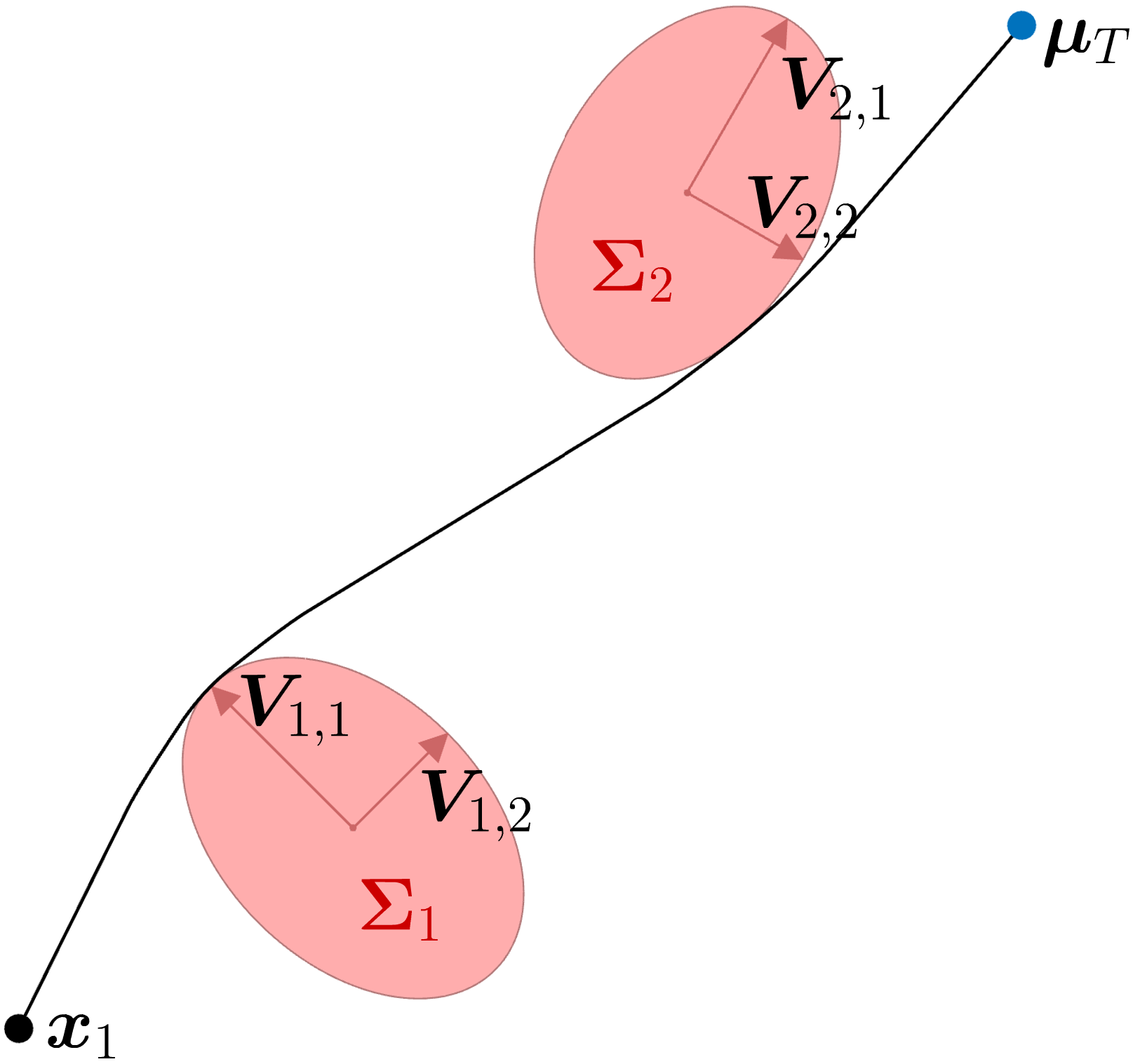
By taking as example a point-mass system, iLQR can be used to solve an ellipsoidal obstacle avoidance problem with the cost (typically used with other costs, see Fig. 21 for an example). We first define a ReLU-like function and its gradient as (see also Fig. 17 - right )
| f^{\text{\tiny avoid}}(d)=\begin{cases}0,&\text{if}\ d>1\\ 1-d,&\text{otherwise}\end{cases},\quad\quad g^{\text{\tiny avoid}}(d)=\begin{cases}0,\hskip 17.071654pt&\text{if}\ d>1\\ -1,&\text{otherwise}\end{cases}, |
that we exploit to define \bm{f}(\bm{x}_{t}) and \bm{J}(\bm{x}_{t}) in ( 98 ) as
| \displaystyle\bm{f}(\bm{x}_{t}) | \displaystyle=f^{\text{\tiny avoid}}\Big(e(\bm{x}_{t})\Big),\quad\quad\bm{J}(\bm{x}_{t})=2\;g^{\text{\tiny avoid}}\Big(e(\bm{x}_{t})\Big)\;{(\bm{x}_{t}-\bm{\mu})}^{\scriptscriptstyle\top}\;\bm{\Sigma}^{-1}, | ||
| \displaystyle\text{with}\quad e(\bm{x}_{t}) | \displaystyle={(\bm{x}_{t}-\bm{\mu})}^{\scriptscriptstyle\top}\bm{\Sigma}^{-1}(\bm{x}_{t}-\bm{\mu}). |
In the above, \bm{f}(\bm{x}) defines a continuous function that is 0 outside the obstacle boundaries and 1 at the center of the obstacle. The ellipsoid is defined by a center \bm{\mu} and a shape \bm{\Sigma}=\bm{V}\bm{V}^{\scriptscriptstyle\top} , where \bm{V} is a horizontal concatenation of vectors \bm{V}_{i} describing the principal axes of the ellipsoid, see Fig. 21 .
A similar principle can be applied to robot manipulators by composing forward kinematics and obstacle avoidance functions.
7.5.8 Maintaining a desired distance to an object
The obstacle example above can easily be extended to the problem of maintaining a desired distance to an object, which can also typically used with other objectives. We first define a function and a gradient
| f^{\text{\tiny dist}}(d)=1-d,\quad\quad g^{\text{\tiny dist}}(d)=-1, |
that we exploit to define \bm{f}(\bm{x}_{t}) and \bm{J}(\bm{x}_{t}) in ( 98 ) as
| \displaystyle\bm{f}(\bm{x}_{t}) | \displaystyle=f^{\text{\tiny dist}}\Big(e(\bm{x}_{t})\Big),\quad\quad\bm{J}(\bm{x}_{t})=-\frac{2}{r^{2}}{(\bm{x}_{t}-\bm{\mu})}^{\scriptscriptstyle\top}, | ||
| \displaystyle\text{with}\quad e(\bm{x}_{t}) | \displaystyle=\frac{1}{r^{2}}{(\bm{x}_{t}-\bm{\mu})}^{\scriptscriptstyle\top}(\bm{x}_{t}-\bm{\mu}). |
In the above, \bm{f}(\bm{x}) defines a continuous function that is 0 on a sphere of radius r centered on the object (defined by a center \bm{\mu} ), and increasing/decreasing when moving away from this surface in one direction or the other.
7.5.9 Manipulability tracking
Skills transfer can exploit manipulability ellipsoids in the form of geometric descriptors representing the skills to be transferred to the robot. As these ellipsoids lie on symmetric positive definite (SPD) manifolds, Riemannian geometry can be used to learn and reproduce these descriptors in a probabilistic manner [ 3 ] .
Manipulability ellipsoids come in different flavors. They can be defined for either positions or forces (including the orientation/rotational part). Manipulability can be described at either kinematic or dynamic levels, for either open or closed linkages (e.g., for bimanual manipulation or in-hand manipulation), and for either actuated or non-actuated joints [ 13 ] . This large set of manipulability ellipsoids provide rich descriptors to characterize robot skills for robots with legs and arms.
Manipulability ellipsoids are helpful descriptors to handle skill transfer problems involving dissimilar kinematic chains, such as transferring manipulation skills between humans and robots, or between two robots with different kinematic chains or capabilities. In such transfer problems, imitation at joint angles level is not possible due to the different structures, and imitation at end-effector(s) level is limited, because it does not encapsulate postural information, which is often an essential aspect of the skill that we would like to transfer. Manipulability ellipsoids provide intermediate descriptors that allows postural information to be transferred indirectly, with the advantage that it allows different embodiments and capabilities to be considered in the skill transfer process.
The manipulability ellipsoid \bm{M}(\bm{x})=\bm{J}(\bm{x}){\bm{J}(\bm{x})}^{\scriptscriptstyle\top} is a symmetric positive definite matrix representing the manipulability at a given point on the kinematic chain defined by a forward kinematics function \bm{f}(\bm{x}) , given the joint angle posture \bm{x} , where \bm{J}(\bm{x}) is the Jacobian of \bm{f}(\bm{x}) . The determinant of \bm{M}(\bm{x}) is often used as a scalar manipulability index indicating the volume of the ellipsoid [ 15 ] , with the drawback of ignoring the specific shape of this ellipsoid.
In [ 5 ] , we showed that a geometric cost on manipulability can alternatively be defined with the geodesic distance
| \displaystyle c | \displaystyle=\|\bm{A}\|^{2}_{\text{F}},\quad\text{with}\quad\bm{A}=\log\!\big(\bm{S}^{\frac{1}{2}}\bm{M}(\bm{x})\bm{S}^{\frac{1}{2}}\big), | ||
| \displaystyle\iff\;c | \displaystyle=\text{trace}(\bm{A}\bm{A}^{\scriptscriptstyle\top})=\sum_{i}\text{trace}(\bm{A}_{i}\bm{A}_{i}^{\scriptscriptstyle\top})=\sum_{i}\bm{A}_{i}^{\scriptscriptstyle\top}\bm{A}_{i}={\text{vec}(\bm{A})}^{\scriptscriptstyle\top}\text{vec}(\bm{A}), |
where \bm{S} is the desired manipulability matrix to reach, \log(\cdot) is the logarithm matrix function, and \|\cdot\|_{\text{F}} is a Frobenius norm. By exploiting the trace properties, we can see that ( 100 ) can be expressed in a quadratic form, where the vectorization operation \text{vec}(\bm{A}) can be computed efficiently by exploiting the symmetry of the matrix \bm{A} . This is implemented by keeping only the lower half of the matrix, with the elements below the diagonal multiplied by a factor \sqrt{2} .
The derivatives of ( 100 ) with respect to the state \bm{x} and control commands \bm{u} can be computed numerically (as in the provided example), analytically (by following an approach similar to the one presented in [ 5 ] ), or by automatic differentiation. The quadratic form of ( 100 ) can be exploited to solve the iLQR problem with Gauss–Newton optimization, by using Jacobians (see description in Section 4.1 within the context of inverse kinematics). Marić et al. demonstrated the advantages of a geometric cost as in ( 100 ) for planning problems, by comparing it to alternative widely used metrics such as the manipulability index and the dexterity index [ 7 ] .
Note here that manipulability can be defined at several points of interest, including endeffectors and centers of mass. Figure 22 presents a simple example with a bimanual robot. Manipulability ellipsoids can also be exploited as descriptors for object affordances, by defining manipulability at the level of specific points on objects or tools held by the robot. For example, we can consider a manipulability ellipsoid at the level of the head of a hammer. When the robot grasps the hammer, its endeffector is extended so that the head of the hammer becomes the extremity of the kinematic chain. In this situation, the different options that the robot has to grasp the hammer will have an impact on the resulting manipulability at the head of the hammer. Thus, grabbing the hammer at the extremity of the handle will improve the resulting manipulability. Such descriptors offer promises for learning and optimization in manufacturing environments, in order to let robots automatically determine the correct ways to employ tools, including grasping points and body postures.
The above iLQR approach, with a geodesic cost on SPD manifolds, has been presented for manipulability ellipsoids, but it can be extended to other descriptors represented as ellipsoids. In particular, stiffness, feedback gains, inertia, and centroidal momentum have similar structures. For the latter, the centroidal momentum ellipsoid quantifies the momentum generation ability of the robot [ 11 ] , which is another useful descriptor for robotics skills. Similarly to manipulability ellipsoids, it is constructed from Jacobians, which are in this case the centroidal momentum matrices mapping the joint angle velocities to the centroidal momentum, which sums over the individual link momenta after projecting each to the robot’s center of mass.
The approach can also be extended to other forms of symmetric positive definite matrices, such as kernel matrices used in machine learning algorithms to compute similarities, or graph graph Laplacians (a matrix representation of a graph that can for example be used to construct a low dimensional embedding of a graph).
7.6 iLQR with control primitives
The use of control primitives can be extended to iLQR, by considering \Delta\bm{u}=\bm{\Psi}\Delta\bm{w} . For problems with quadratic cost on \bm{f}(\bm{x}_{t}) (see previous Section), the update of the weights vector is then given by
| \Delta\bm{\hat{w}}\!=\!{\Big(\bm{\Psi}^{\!{\scriptscriptstyle\top}}\bm{S}_{\bm{u}}^{\scriptscriptstyle\top}\bm{J}(\bm{x})^{\scriptscriptstyle\top}\bm{Q}\bm{J}(\bm{x})\bm{S}_{\bm{u}}\bm{\Psi}+\bm{\Psi}^{\!{\scriptscriptstyle\top}}\bm{R}\,\bm{\Psi}\Big)}^{\!\!-1}\Big(-\bm{\Psi}^{\!{\scriptscriptstyle\top}}\bm{S}_{\bm{u}}^{\scriptscriptstyle\top}\bm{J}(\bm{x})^{\scriptscriptstyle\top}\bm{Q}\bm{f}(\bm{x})-\bm{\Psi}^{\!{\scriptscriptstyle\top}}\bm{R}\,\bm{u}\Big). |
For a 5-link kinematic chain, by setting the coordination matrix in ( 58 ) as
| \bm{C}=\begin{bmatrix}-1&0&0\\ 2&0&0\\ -1&0&0\\ 0&1&0\\ 0&0&1\end{bmatrix}, |
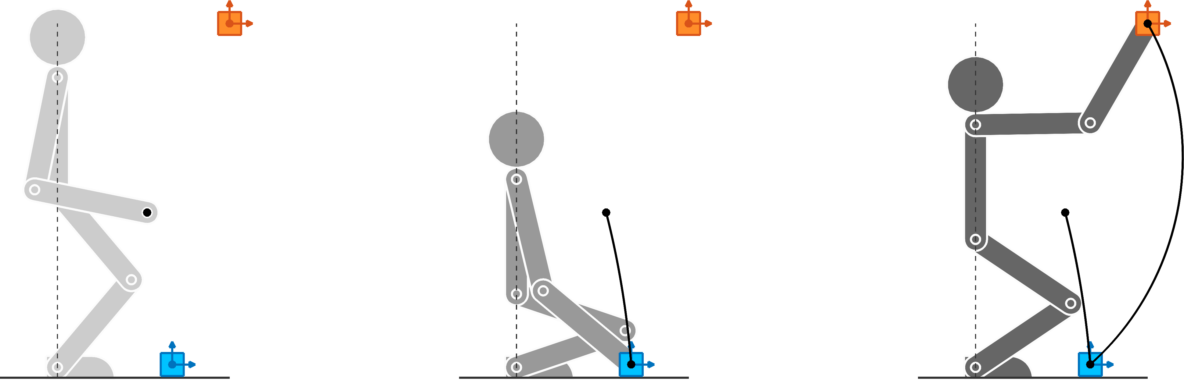
the first three joints are coordinated such that the third link is always oriented in the same direction, while the last two joints can move independently. Figure 23 shows an example for a reaching task, with the 5-link kinematic chain depicting a humanoid robot that needs to keep its torso upright.
Note also that the iLQR updates in ( 101 ) can usually be computed faster than in the original formulation, since a matrix of much smaller dimension needs to be inverted.
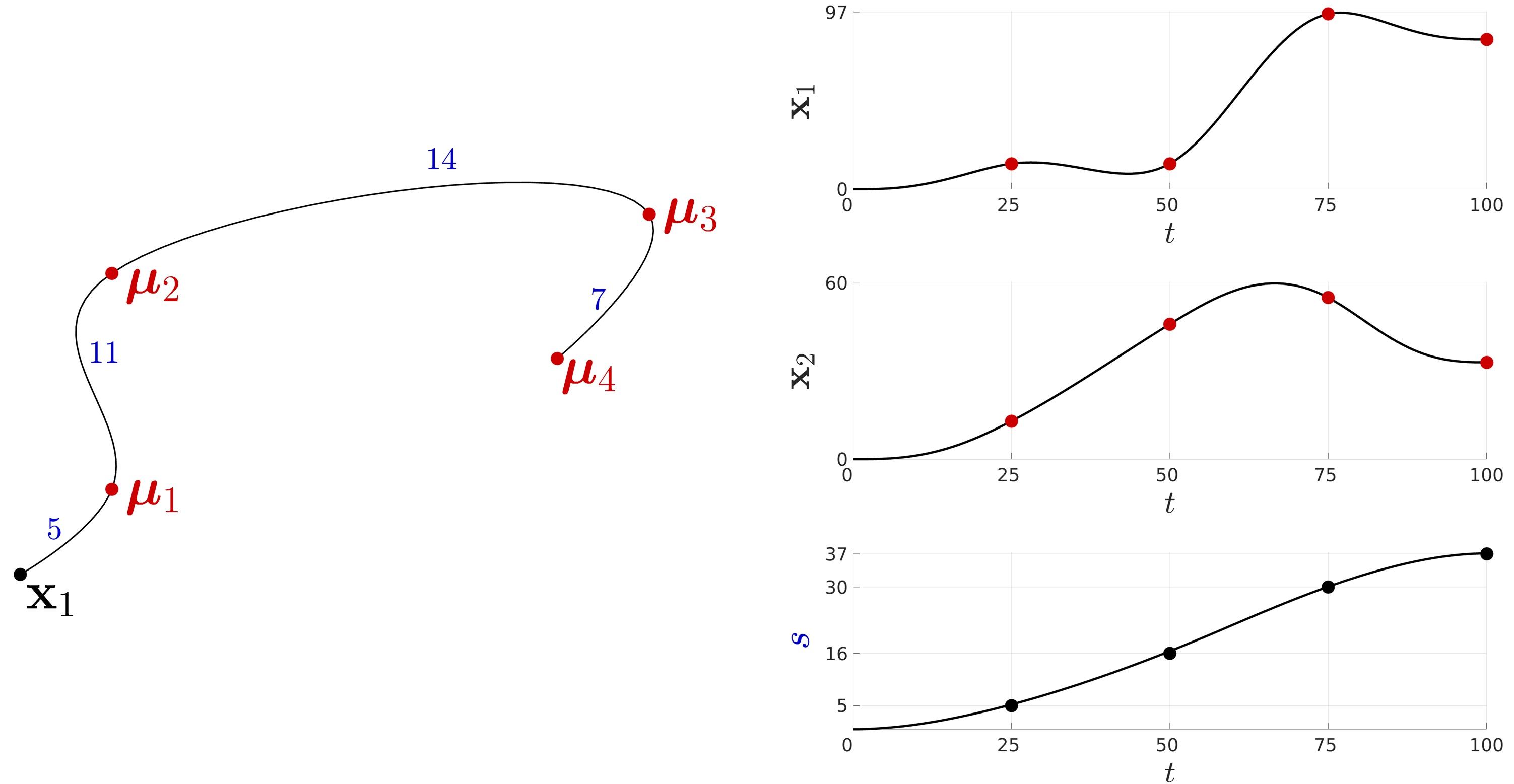
7.7 iLQR for spacetime optimization
We define a phase variable s_{t} starting from s_{1}=0 at the beginning of the movement. With an augmented state \bm{x}_{t}={[\mathbf{x}_{t}^{\scriptscriptstyle\top},s_{t}]}^{\scriptscriptstyle\top} and control command \bm{u}_{t}={[{\bm{u}^{\mathbf{x}}_{t}}^{\scriptscriptstyle\top},u^{s}_{t}]}^{\scriptscriptstyle\top} , we define the evolution of the system \bm{x}_{t+1}=\bm{d}(\bm{x}_{t},\bm{u}_{t}) as
| \displaystyle\mathbf{x}_{t+1} | \displaystyle=\mathbf{A}_{t}\mathbf{x}_{t}+\mathbf{B}_{t}\bm{u}^{\mathbf{x}}_{t}\,u^{s}_{t}, | ||
| \displaystyle s_{t+1} | \displaystyle=s_{t}+u^{s}_{t}. |
Its first order Taylor expansion around \bm{\hat{x}},\bm{\hat{u}} provides the linear system
| \displaystyle\underbrace{\begin{bmatrix}\textstyle\Delta\mathbf{x}_{t+1}\\ \textstyle\Delta s_{t+1}\end{bmatrix}}_{\Delta\bm{x}_{t+1}} | \displaystyle=\underbrace{\begin{bmatrix}\textstyle\mathbf{A}_{t}&\bm{0}\\ \textstyle\bm{0}&1\end{bmatrix}}_{\bm{A}_{t}}\underbrace{\begin{bmatrix}\textstyle\Delta\mathbf{x}_{t}\\ \textstyle\Delta s_{t}\end{bmatrix}}_{\Delta\bm{x}_{t}}+\underbrace{\begin{bmatrix}\textstyle\mathbf{B}_{t}u^{s}_{t}&\mathbf{B}_{t}\bm{u}^{\mathbf{x}}_{t}\\ \textstyle\bm{0}&1\end{bmatrix}}_{\bm{B}_{t}}\underbrace{\begin{bmatrix}\textstyle\Delta\bm{u}^{\mathbf{x}}_{t}\\ \textstyle\Delta u^{s}_{t}\end{bmatrix}}_{\Delta\bm{u}_{t}}, |
with Jacobian matrices \bm{A}_{t}\!=\!\frac{\partial\bm{d}}{\partial\bm{x}_{t}} , \bm{B}_{t}\!=\!\frac{\partial\bm{d}}{\partial\bm{u}_{t}} . Note that in the above equations, we used here the notation \mathbf{x}_{t} and \bm{x}_{t} to describe the standard state and augmented state, respectively. We similarly used \{\mathbf{A}_{t},\mathbf{B}_{t}\} and \{\bm{A}_{t},\bm{B}_{t}\} (with slanted font) for standard linear system and augmented linear system.
Figure 24 shows a viapoints task example in which both path and duration are optimized (convergence after 10 iterations when starting from zero commands). The example uses a double integrator as linear system defined by constant \mathbf{A}_{t} and \mathbf{B}_{t} matrices.
7.8 iLQR with offdiagonal elements in the precision matrix
Spatial and/or temporal constraints can be considered by setting \left[\begin{smallmatrix}\bm{I}&-\bm{I}\\ -\bm{I}&\bm{I}\end{smallmatrix}\right] in the corresponding entries of the precision matrix \bm{Q} . With this formulation, we can constrain two positions to be the same without having to predetermine the position at which the two should meet. Indeed, we can see that a cost c\!=\!\left[\begin{smallmatrix}x_{i}\\ x_{j}\end{smallmatrix}\right]^{\scriptscriptstyle\top}\left[\begin{smallmatrix}1&-1\\ -1&1\end{smallmatrix}\right]\left[\begin{smallmatrix}x_{i}\\ x_{j}\end{smallmatrix}\right]\!=\!(x_{i}-x_{j})^{2} is minimized when x_{i}\!=\!x_{j} .
Such cost can for example be used to define costs on object affordances, see Fig. 25 for an example.
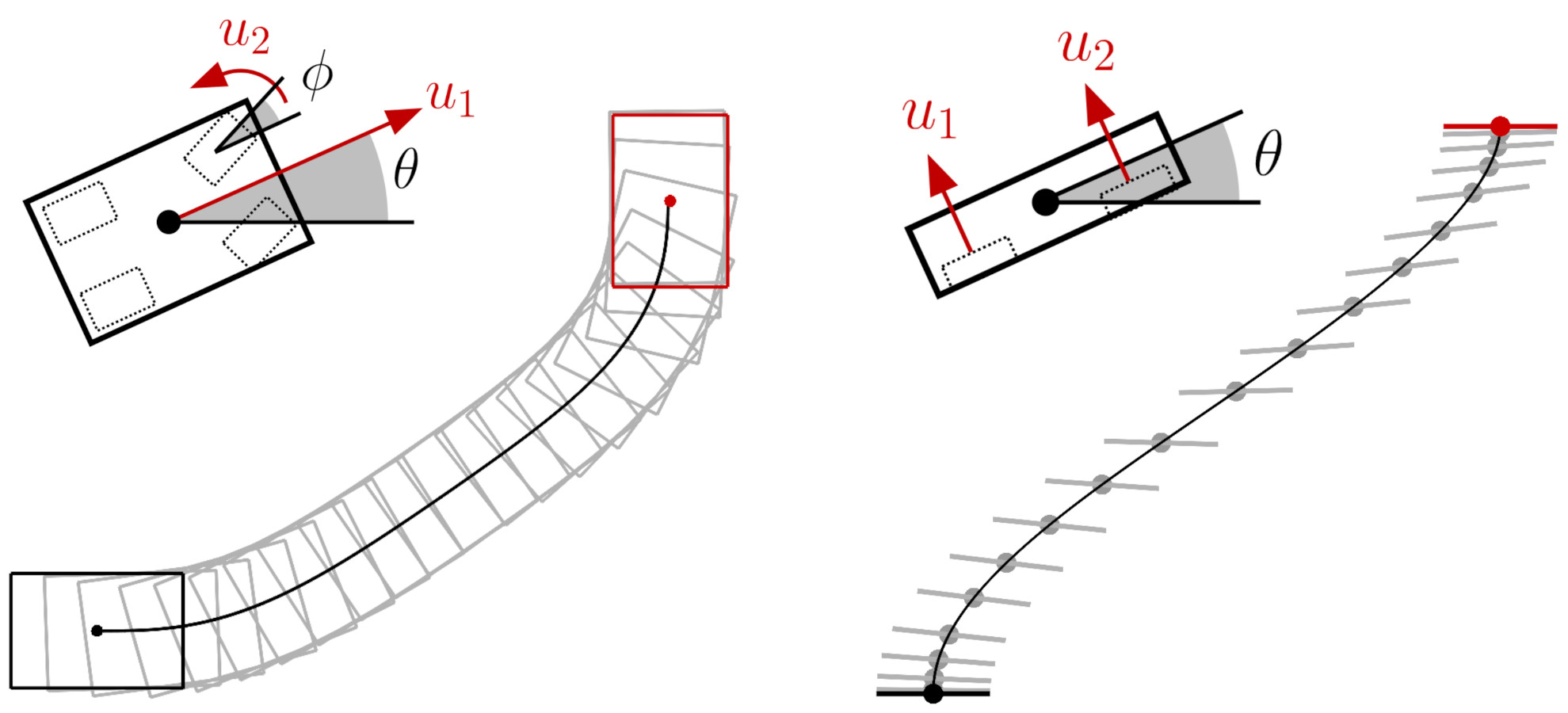
7.9 Car steering
Velocity Control Input
A car motion with position
(x_{1},x_{2})
, car orientation
\theta
, and front wheels orientation
\phi
(see Fig.
26
-
left
) is characterized by equations
| \dot{x}_{1}=u_{1}\cos(\theta),\quad\dot{x}_{2}=u_{1}\sin(\theta),\quad\dot{\theta}=\frac{u_{1}}{\ell}\tan(\phi),\quad\dot{\phi}=u_{2}, |
where \ell is the distance between the front and back axles, u_{1} is the back wheels velocity command and u_{2} is the front wheels steering velocity command. Its first order Taylor expansion around (\hat{\theta},\hat{\phi},\hat{u}_{1}) is
| \footnotesize\begin{bmatrix}\Delta\dot{x}_{1}\\ \Delta\dot{x}_{2}\\ \Delta\dot{\theta}\\ \Delta\dot{\phi}\end{bmatrix}=\begin{bmatrix}0&0&-\hat{u}_{1}\sin(\hat{\theta})&0\\ 0&0&\hat{u}_{1}\cos(\hat{\theta})&0\\ 0&0&0&\frac{\hat{u}_{1}}{\ell}(\tan(\hat{\phi})^{2}\!+\!1)\\ 0&0&0&0\end{bmatrix}\begin{bmatrix}\Delta x_{1}\\ \Delta x_{2}\\ \Delta\theta\\ \Delta\phi\end{bmatrix}+\footnotesize\begin{bmatrix}\cos(\hat{\theta})&0\\ \sin(\hat{\theta})&0\\ \frac{1}{\ell}\tan(\hat{\phi})&0\\ 0&1\end{bmatrix}\begin{bmatrix}\Delta u_{1}\\ \Delta u_{2}\end{bmatrix}, |
which can then be converted to a discrete form with (
117
).
Acceleration Control Input
A car motion with position
(x_{1},x_{2})
, car orientation
\theta
, and front wheels orientation
\phi
(see Fig.
26
-
left
) is characterized by equations
| \dot{x}_{1}=v\cos(\theta),\quad\dot{x}_{2}=v\sin(\theta),\quad\dot{\theta}=\frac{v}{\ell}\tan(\phi),\quad\dot{v}=u_{1},\quad\dot{\phi}=u_{2}, |
where \ell is the distance between the front and back axles, u_{1} is the back wheels acceleration command and u_{2} is the front wheels steering velocity command. Its first order Taylor expansion around (\hat{\theta},\hat{\phi},\hat{v}) is
| \footnotesize\begin{bmatrix}\Delta\dot{x}_{1}\\ \Delta\dot{x}_{2}\\ \Delta\dot{\theta}\\ \Delta\dot{v}\\ \Delta\dot{\phi}\end{bmatrix}=\begin{bmatrix}0&0&-\hat{v}\sin(\hat{\theta})&\cos(\hat{\theta})&0\\ 0&0&\hat{v}\cos(\hat{\theta})&\sin(\hat{\theta})&0\\ 0&0&0&\frac{1}{\ell}\tan(\hat{\phi})&\frac{\hat{v}}{\ell}(\tan(\hat{\phi})^{2}\!+\!1)\\ 0&0&0&0&0\\ 0&0&0&0&0\end{bmatrix}\begin{bmatrix}\Delta x_{1}\\ \Delta x_{2}\\ \Delta\theta\\ \Delta v\\ \Delta\phi\end{bmatrix}+\footnotesize\begin{bmatrix}0&0\\ 0&0\\ 0&0\\ 1&0\\ 0&1\end{bmatrix}\begin{bmatrix}\Delta u_{1}\\ \Delta u_{2}\end{bmatrix}, |
which can then be converted to a discrete form with ( 117 ).
7.10 Bicopter
A planar bicopter of mass m and inertia I actuated by two propellers at distance \ell (see Fig. 26 - right ) is characterized by equations
| \ddot{x}_{1}=-\frac{1}{m}(u_{1}+u_{2})\sin(\theta),\quad\ddot{x}_{2}=\frac{1}{m}(u_{1}+u_{2})\cos(\theta)-g,\quad\ddot{\theta}=\frac{\ell}{I}(u_{1}-u_{2}), |
with acceleration g\!=\!9.81 due to gravity. Its first order Taylor expansion around (\hat{\theta},\hat{u}_{2},\hat{u}_{2}) is
| \footnotesize\begin{bmatrix}\Delta\dot{x}_{1}\\ \Delta\dot{x}_{2}\\ \Delta\dot{\theta}\\ \Delta\ddot{x}_{1}\\ \Delta\ddot{x}_{2}\\ \Delta\ddot{\theta}\end{bmatrix}=\begin{bmatrix}0&0&0&1&0&0\\ 0&0&0&0&1&0\\ 0&0&0&0&0&1\\ 0&0&-\frac{1}{m}(\hat{u}_{1}+\hat{u}_{2})\cos(\hat{\theta})&0&0&0\\ 0&0&-\frac{1}{m}(\hat{u}_{1}+\hat{u}_{2})\sin(\hat{\theta})&0&0&0\\ 0&0&0&0&0&0\end{bmatrix}\begin{bmatrix}\Delta x_{1}\\ \Delta x_{2}\\ \Delta\theta\\ \Delta\dot{x}_{1}\\ \Delta\dot{x}_{2}\\ \Delta\dot{\theta}\end{bmatrix}+\footnotesize\begin{bmatrix}0&0\\ 0&0\\ 0&0\\ -\frac{1}{m}\sin(\hat{\theta})&-\frac{1}{m}\sin(\hat{\theta})\\ \frac{1}{m}\cos(\hat{\theta})&\frac{1}{m}\cos(\hat{\theta})\\ \frac{\ell}{I}&-\frac{\ell}{I}\end{bmatrix}\begin{bmatrix}\Delta u_{1}\\ \Delta u_{2}\end{bmatrix}, |
which can then be converted to a discrete form with ( 117 ).