Exercise 2
Movement primitives, Newton's Method

1. Understanding basis functions

You will find below a visualization of basis functions defined by the function build_basis_function which takes nb_data (number of timesteps) and nb_fct (number of basis functions) as arguments and returns phi the matrix of basis functions.

1. Visualize what happens when you change the parameter nb_fct.
2. Visualize what happens when you change the parameter param_lambda.
3. Change the function below to plot Bézier basis functions (you can compare your result to Figure 1 in the RCFS documentation).

param_lambda = 1e2 nb_data = 100 nb_fct = 10 def build_basis_function(nb_data, nb_fct): t = np.linspace(0,1,nb_data).reshape((-1,1)) tMu = np.linspace( t[0] , t[-1] , nb_fct ) phi = np.exp( - param_lambda * (t.T - tMu)**2 ).T return phi phi = build_basis_function(nb_data, nb_fct) fig,ax = plt.subplots(figsize=(5,5)) ax.plot(np.linspace(0,1,nb_data), phi) ax.set_xlabel('time(s)') ax.set_ylabel('basis functions') fig.tight_layout() fig

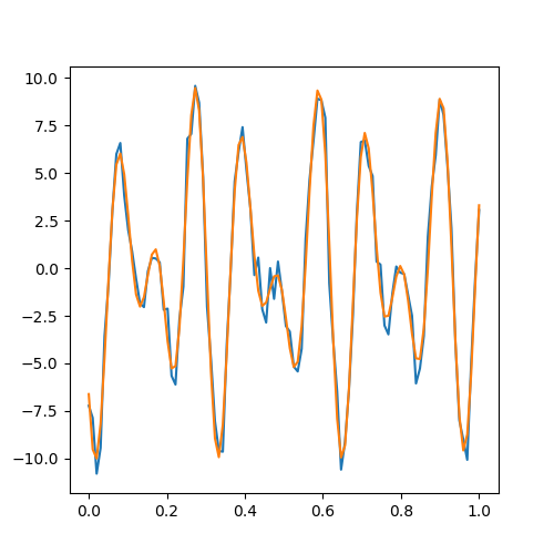
2. Regression with basis functions \bm{x} = \bm{\Phi} \bm{w}

We can use basis functions to encode trajectories in a compact way. Such encoding aims at encoding the movement as a weighted superposition of simpler movements, whose compression aims at working in a subspace of reduced dimensionality, while denoising the signal and capturing the essential aspects of a movement. We first generate a noisy time trajectory using the function generate_data.

1. Run the code below to plot the function below in your workspace by choosing an appropriate noise_scale. We will use \bm{x} as our dataset vector.

noise_scale = 1. # change this to the noise level you want nb_data = 100 def generate_data(t): return 10*np.sin(50*t+10)*np.cos(10*t) t = np.linspace(0,1,nb_data) x = generate_data(t) + np.random.randn(nb_data)*noise_scale
fig,ax = plt.subplots(figsize=(5,5)) ax.plot(t,x) ax.set_xlabel('t') ax.set_ylabel('x') fig

2. Using the implemented build_basis_function, write a function that takes the basis function matrix \bm{\phi} and determines the Bézier curve parameters \bm{w} that represents the data the best in least-square sense.

nbFct = 30 psi = build_basis_function(nb_data,nbFct) def estimate_w(x, psi): # w = # Implement here: Estimation of superposition weights from data return w w = estimate_w(x, psi) print(w.shape) # verify the dimension of this to be equal to nbFct

3. Verify your estimation of \bm{w} by reconstructing the data using \bm{\hat{x}} = \bm{\Phi} \bm{w} and plot.

def reconstruct(w, psi): # x_hat = # Implement here: Reconstruction data return x_hat x_hat = reconstruct(w, psi) ax.plot(t, x_hat) fig
Show/hide answer



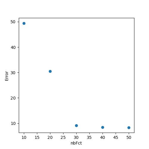
4. We would like to quantify how does the number of basis functions affect the reconstruction. Choose 5 different nb_fct and plot the errors between the original data \bm{x} and the reconstructed data \bm{\hat{x}}.

nbFcts = [] # Implement here: choose 5 different nbFct errors = [] for nbFct in nbFcts: psi = build_basis_function(nb_data, nbFct) w = estimate_w(x, psi) x_hat = reconstruct(w, psi) # errors.append() # Implement here: compute the error between x and x_hat fig,ax = plt.subplots(figsize=(5,5)) ax.plot(nbFcts, errors, 'o') ax.set_xlabel('nbFcts') ax.set_ylabel('Error') fig
Show/hide answer

3. Newton's Method

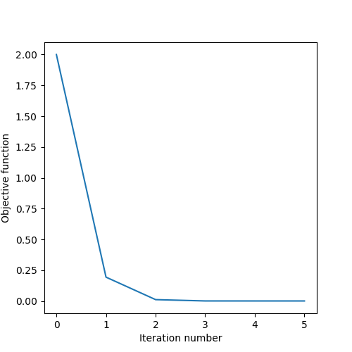
In this exercise, we will implement a Newton's method with a line search. For Newton's method, you can refer to Section 3 of the RCFS documentation and for a backtracking line search algorithm, you can refer to Section 8.4 of the RCFS documentation. The goal is to solve an unconstrained optimization problem using Newton's method and see how line search can affect the convergence. You are given an objective function \bm{x}^2 + \bm{x}^3, its first derivative 2\bm{x} + 3\bm{x}^2 and its second derivative 2+6\bm{x}.

1. Implement Newton's method with a line search and solve the problem.
2. In how many iterations do you get convergence? Plot the cost functions obtained during the iterations and discuss how does the line search affect the results.
3. Change the objective function and its first and second derivatives to solve for another problem.

def objective_function(x): return x**2 + x**3 def first_derivative(x): return 2*x + 3*(x**2) def second_derivative(x): return 2 + 6*x x = 1. cost = objective_function(x) x_log = [x] cost_log = [cost] for i in range(100): # Implement Newton's method here (one line) # search_direction = # Implement line search here (output: alpha) alpha = 1. for j in range(10): # x_trial = # implement a trial x in the direction of search_direction cost_trial = objective_function(x_trial) if cost_trial < cost: break else: alpha = alpha * 0.5 # Convergence check prev_cost = np.copy(cost) x = x + alpha * search_direction cost = objective_function(x) cost_log += [cost] if np.abs(cost-prev_cost) < 1e-6: break x_log.append(x) x_log = np.array(x_log) cost_log = np.array(cost_log) print(x_log)
fig,ax = plt.subplots(figsize=(5,5)) ax.plot(np.arange(0,i+2), cost_log) ax.set_xlabel('Iteration number') ax.set_ylabel('Objective function') fig.tight_layout() fig